The bi-directional slot fed HF antenna isn’t mentioned very often these days for some strange reason. It’s a real shame as it is an excellent antenna that gives high gain through the loop between the frequencies of 14Mhz and 29Mhz.
M0AWS 20m – 10m Slot Fed HF Antenna
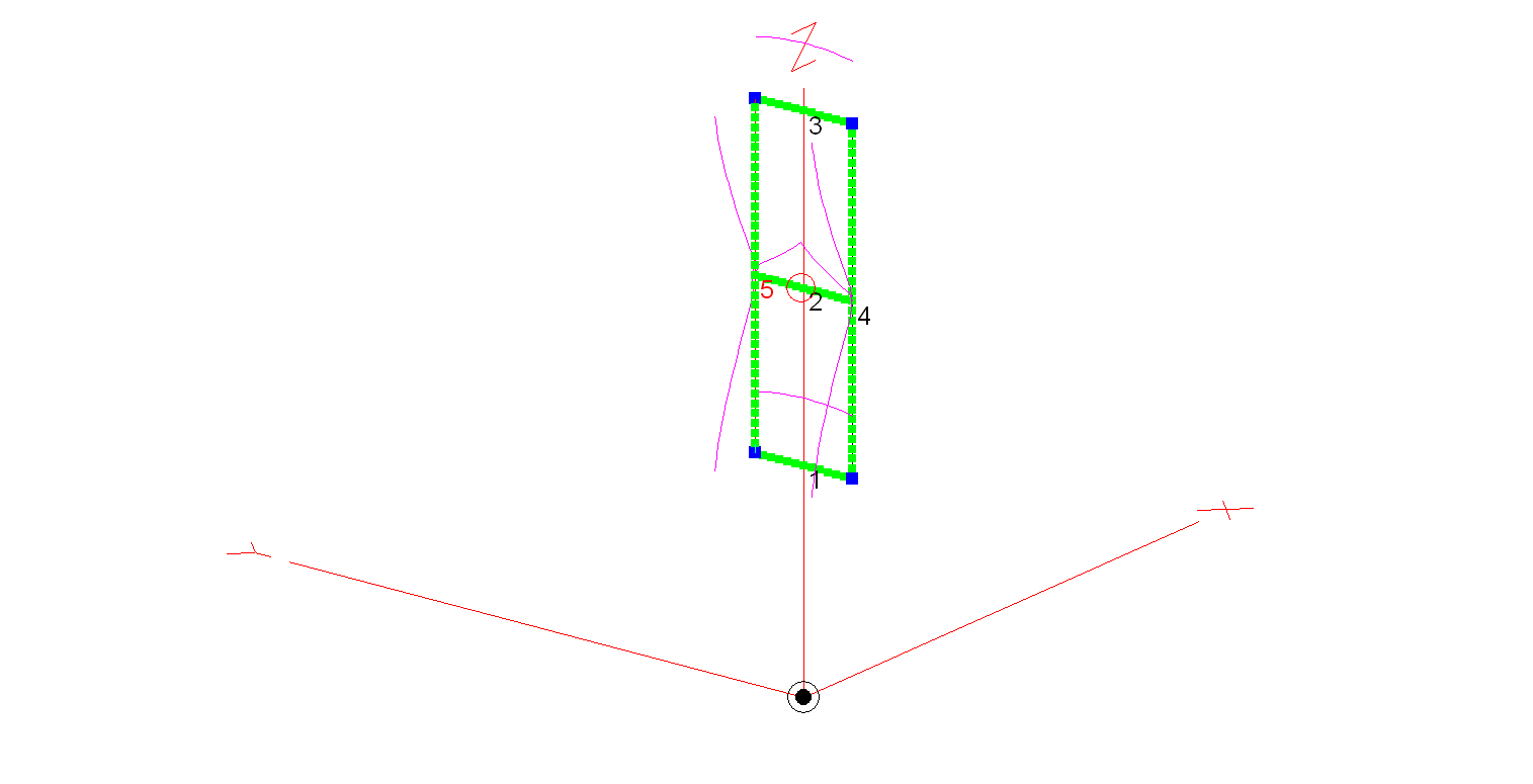
Construction of the antenna is relatively simple, 3 x 3m long horizontal wires and 2 x 9.2m long vertical wires. I’ve modelled the antenna using 20mm diameter copper tubing for the horizontal conductors and 2.5mm wire for the two vertical conductors. Using the 20mm copper tubing provides a rigid platform for the mounting of the antenna on a non-conductive mast whilst reducing weight by using 2.5mm wire for the vertical conductors. You could of course use 20mm copper tubing for all the conductors if you have a non-conductive mast that can handle the weight.
An alternative option is to hang the antenna from a high tree and secure it in position with non-conductive nylon cord. This works very well and makes it extremely easy to manually rotate.
The antenna is fed at the centre of the middle horizontal tube (conductor 2 in the image above) using one of the following methods:
Method 1 – Use a 4:1 Balun and ATU either in the radio/Radio Shack or connected directly to the Balun. Connecting a remote auto ATU to the balun directly at the feed point is the best option as you will then have a perfect 50 Ohm impedance match to the coax cable going back to the radio. (I’ve used my AH-705 and a 4:1 Balun at the feed point in the past with excellent results).
Method 2 – Connect a remote auto ATU directly to the feed point of the antenna and then 50 Ohm coax back to the radio shack. This will provide a perfect SWR match on all bands and works extremely well. (I’ve used my AH-705 remote auto ATU in this configuration as well in the past, again with excellent results and no discernible difference to method 1).
Method 3 – Feed the antenna with 450 Ohm open ladder line and use a 4:1 Balun and ATU in the radio shack to match the antenna to 50 Ohm radios. It’s important to bring the 450 Ohm ladder line away from the feed point horizontally and not vertically downwards. This will then help to protect the radiation pattern.
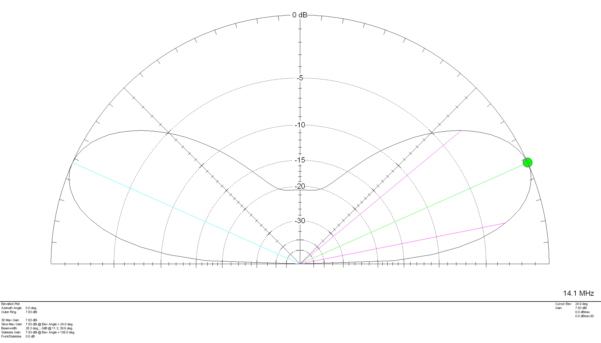
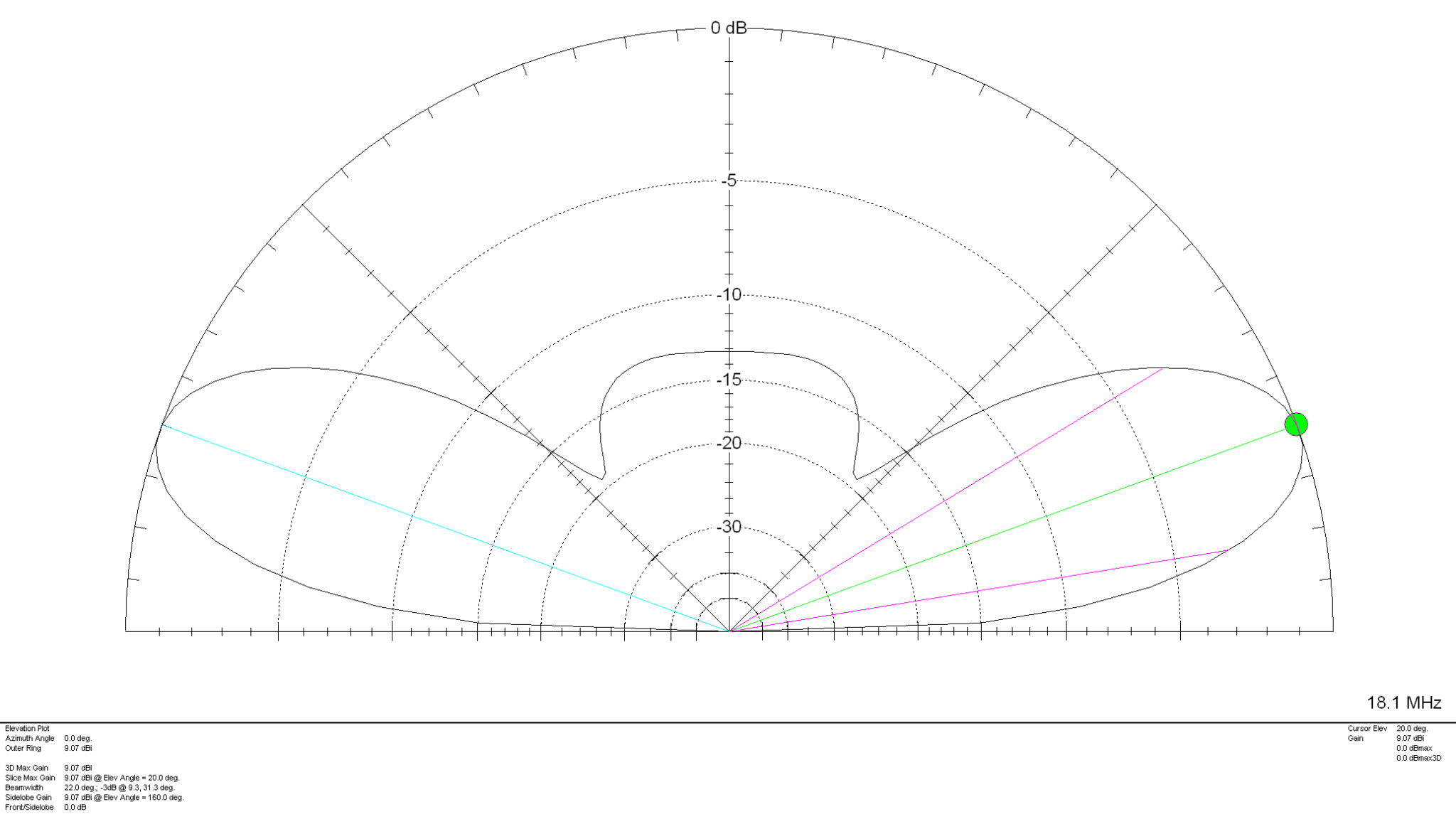
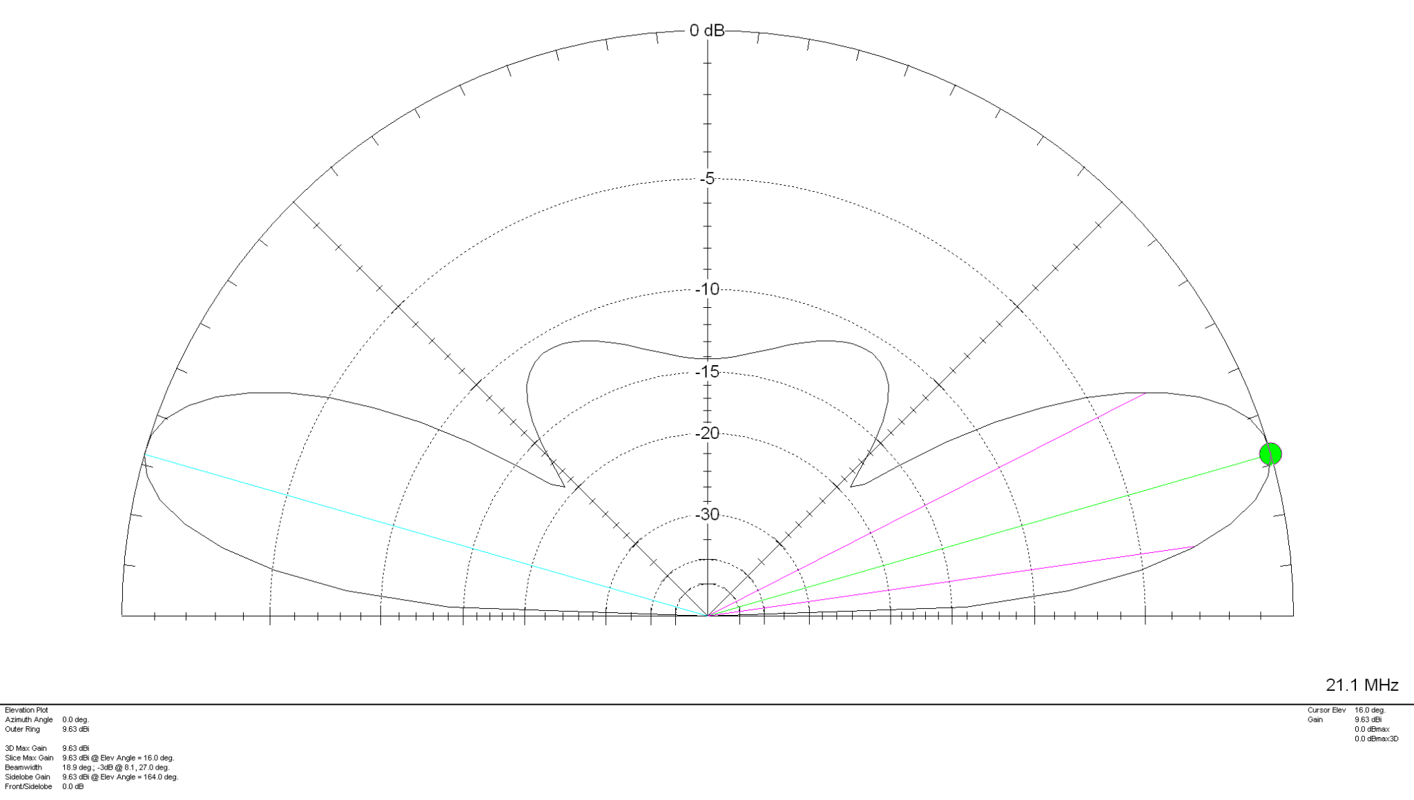
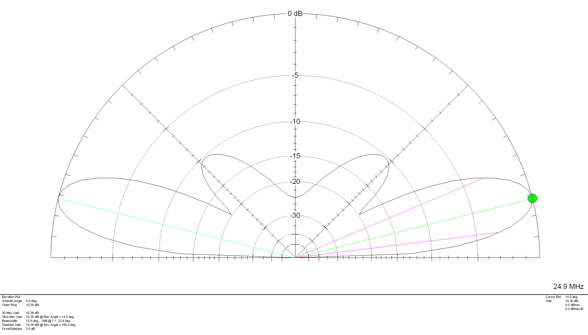
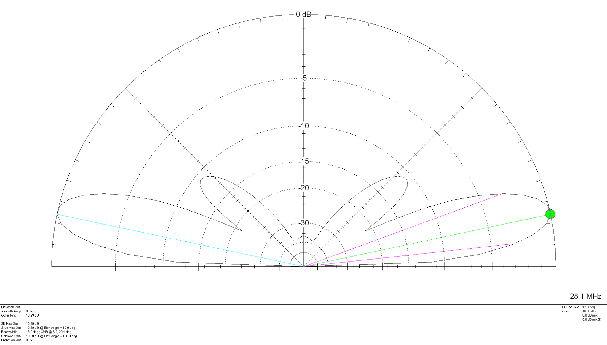
Looking at the 2D Far Field Plots this antenna provides excellent gain at relatively low radiation angles on all bands 20m – 10m making it an ideal antenna for chasing DX.
20m Band 2D Far Field Plot 17m Band 2D Far Field Plot 15m Band 2D Far Field Plot 12m Band 2D Far Field Plot 10m Band 2D Far Field Plot
The gain on each band is as follows:
20m Band – 7.83dBi at 24 Degrees 17m Band – 9.07dBi at 20 Degrees 15m Band – 9.63dBi at 16 Degrees 12m Band – 10.36dBi at 14 Degrees 10m Band – 10.99dBi at 12 Degrees
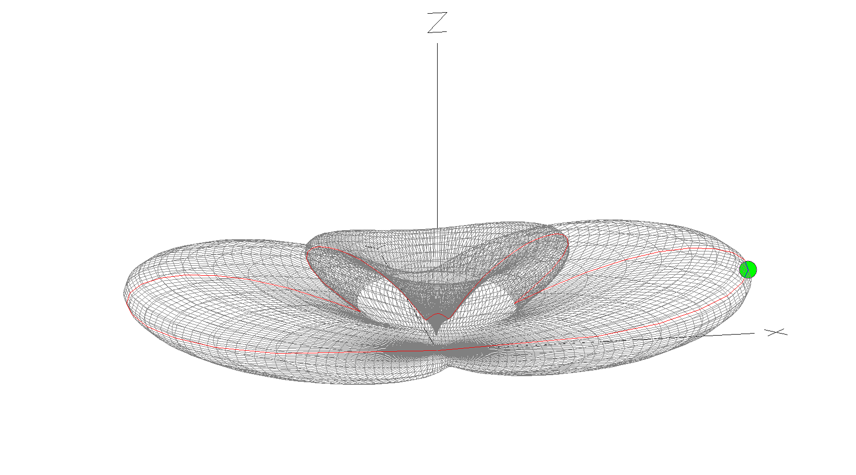
10m Band 3D Far Field Plot
The 10m Band 3D Far Field Plot above shows the typical radiation pattern for the antenna. Maximum radiation is through the loop with very little high angle radiation making it ideal for chasing DX stations. Gain increases as frequency increases however, angle of maximum radiation decreases as frequency increases improving DX capability of the antenna on the higher bands. It’s worth ensuring that the antenna is rotatable as this will then enable you to point the antenna at the DX station to maximise signal strength at the DX end. Pointing this antenna North/South makes it great for working VK/ZL over the North Pole whilst at the same time being able to work South Africa from the UK.
Summary:
Horizontal Wire Lengths: 3m @ 20mm Diameter Vertical Wire Lengths: 9.2m @ 2.5mm Diameter Modelled Height above ground at Centre (Conductor 2): 10.6m Feed Type: 4:1 Balun + ATU / Remote Auto ATU / 450 Ohm Ladder line with 4:1 Balun & ATU
Over the long bank holiday weekend I started putting together my QO-100 ground station. To start with I’ve concentrated solely on the receive path. I’ll start the transmit path once I have the receive path operational at a satisfactory level.
A few weeks ago I purchased a 1.1m off-set dish antenna and a Bullseye LNB. These have been sat in my garage waiting for the weather to improve so that I could start the build in the dry.
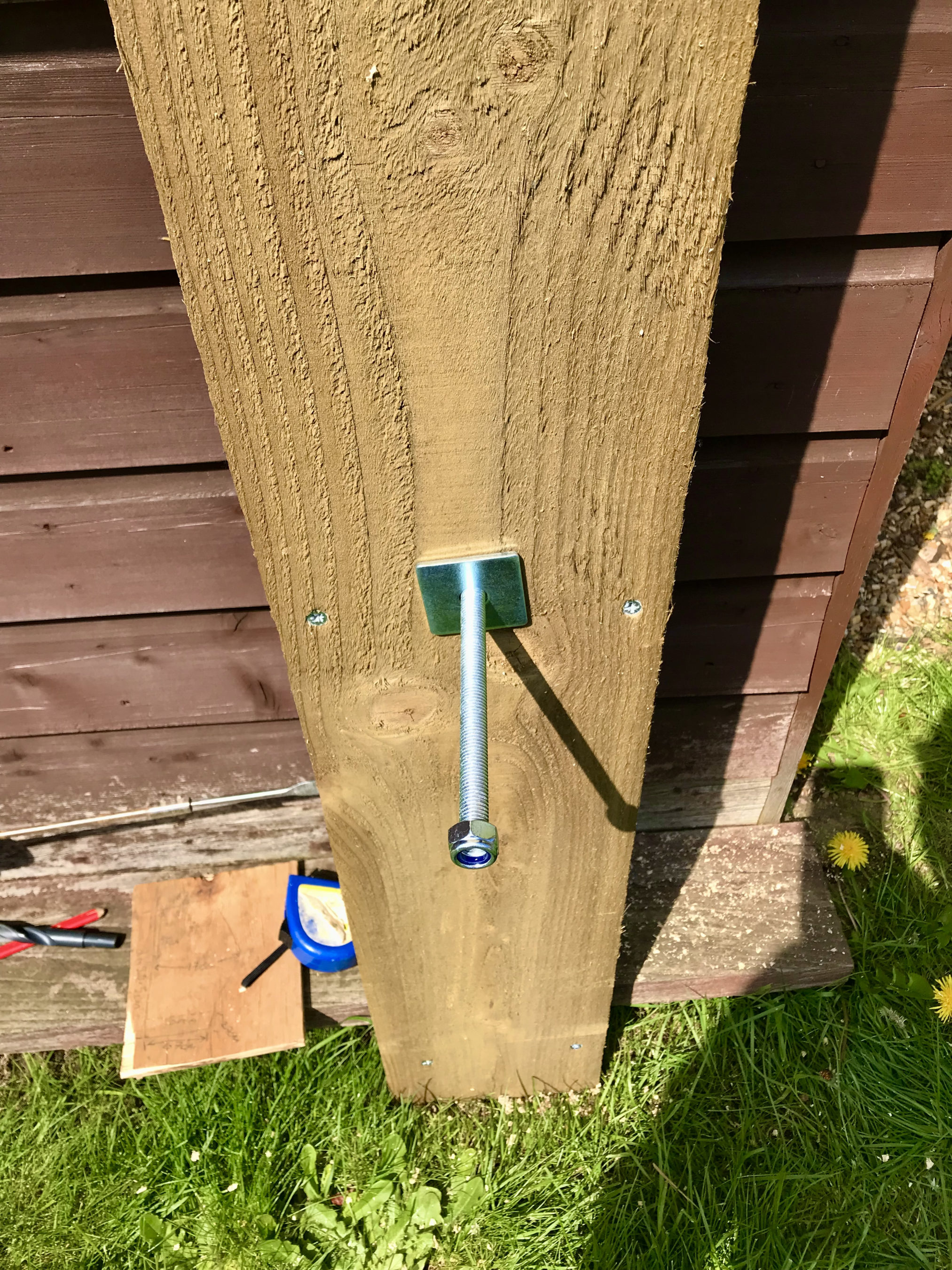
QO-100 Dish MountThrough wall bolt
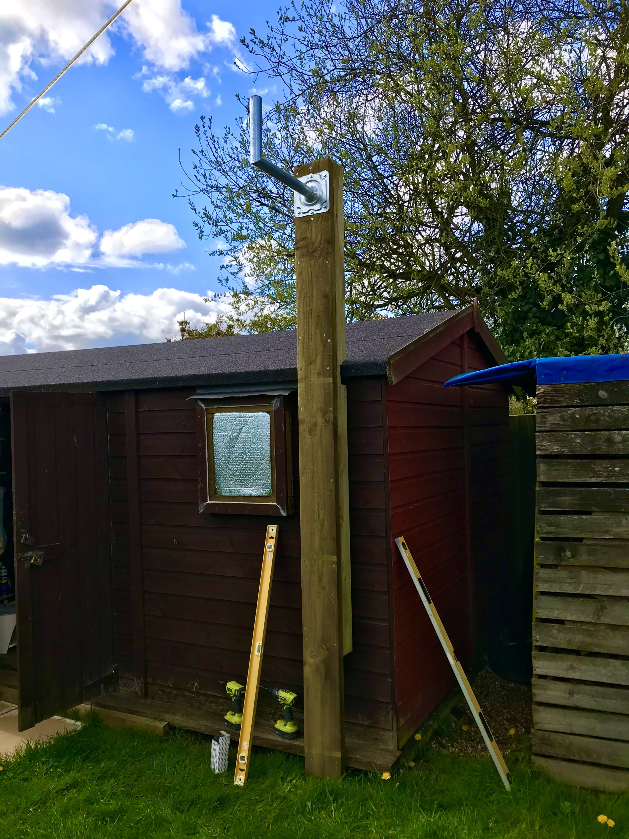
Fortunately we’ve had a mini-summer for the last 2 days and so I started work on getting the dish mount built. Using some timber from the local saw mill I made a braced 3m tall post which I screwed to the side of the cabin to provide a stable fixing platform. I used a couple of threaded bars to bolt through the walls of the cabin to ensure a solid fixing.
Next I mount the metal dish bracket to the top of the wooden post taking the total height up to around 3.2m above ground. This gives plenty of head clearance down below.
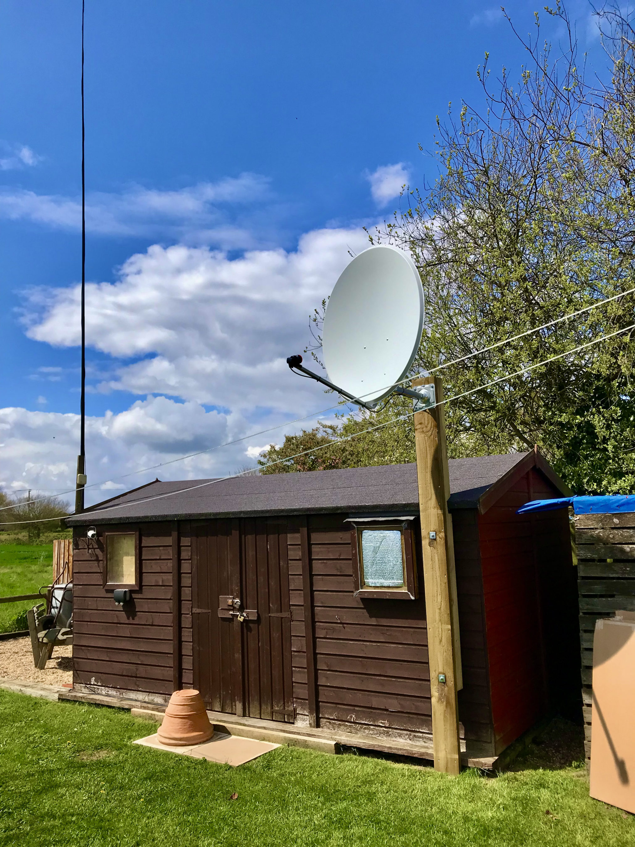
Next I assembled the dish and and attached it to the metal dish bracket at the top of the wooden post.
QO-100 1.1m dish mounted on the 3.2m AGL fixing
Attaching and cabling the Bullseye LNB was an easy job. I used some high quality coax cable that I purchase from the Satellite Superstore when I purchase the dish. I also had to set the LNB skew to -17.8 degrees. The marking on the LNB are tiny and go up in fives and so it’s pretty much impossible to get exactly -17.8 degrees so I turned it to 15 and then a tiny bit. It was as close I could get it!
Next I needed the information on where to point the dish. Fortunately there is a great web app on the BATC website where you can move a pin on a map to your location and all the information you need to align the dish is automagically calculated for you.
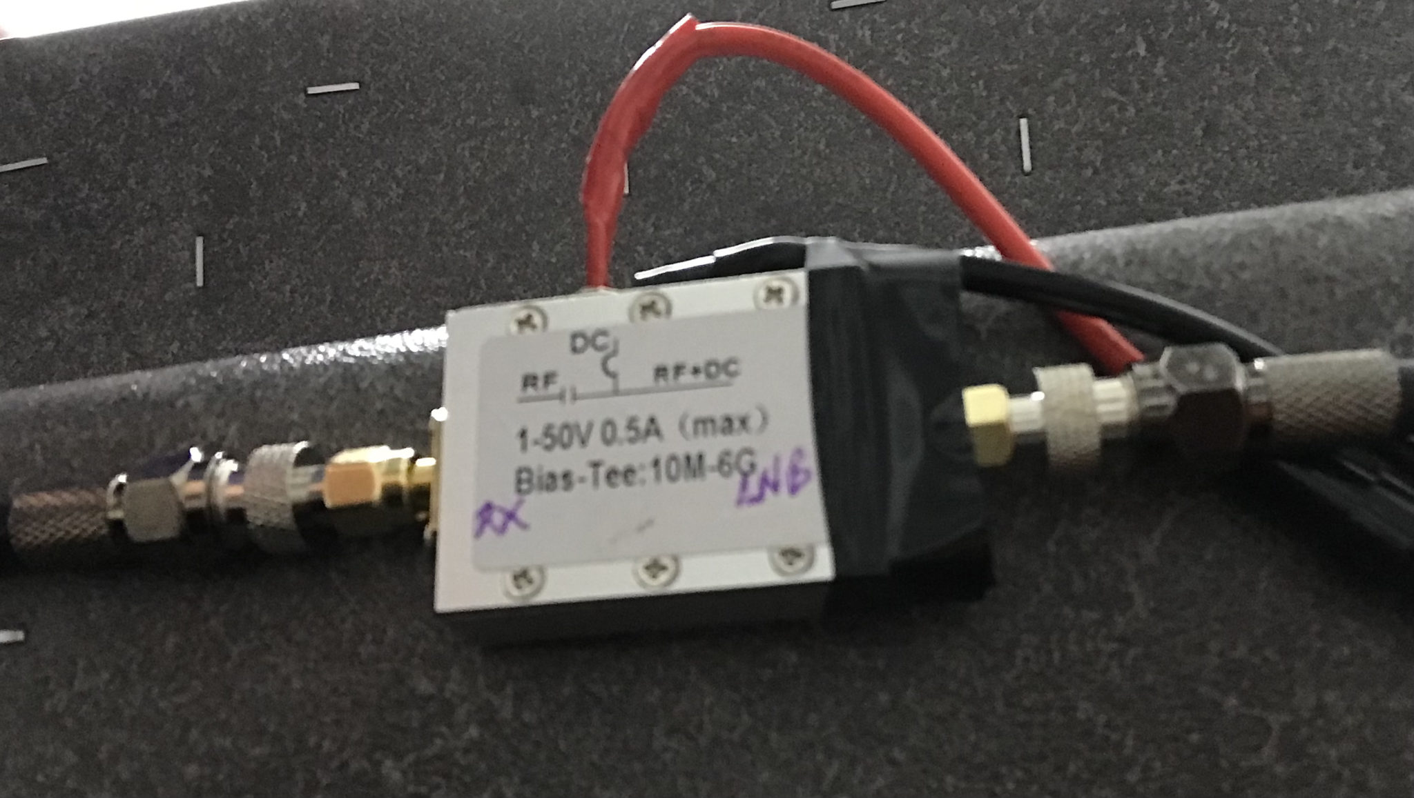
Armed with this info I set about aligning the dish. Getting it as close as possible I lightly locked off the dish and continued getting the coax in to the radio room so that I could connect it to my Funcube Dongle Pro+ (FCD) SDR receiver. Since the LNB needs a 12v DC feed I had to put inline a “Bias Tee” unit. This unit allows you to inject 12v onto the coax going up to the LNB but, stops it from coming back into the receiver. I used a Bias Tee that I purchased from Amazon with the Bullseye LNB.
Bias Tee mounted under the station desk
Connecting the coax to my Funcube Dongle Pro+ I was really pleased to see that I was receiving signals from the satellite perfectly well. I decided to take my laptop up onto the roof of the cabin and see if I could improve the reception further. To my amazement with very tiny changes in elevation and azimuth I was able to improve the QO-100 beacon signal by a further 10dB.
Being pleased with the dish alignment I started to tighten it so that it couldn’t move in the wind. Unfortunately this caused the dish to move a tiny amount which reduced the signal strength. I loosened the bolts off again and realigned the dish once more. This time when I tightened the clamps I did it a bit at a time on each bolt working my way round them so that the dish didn’t move. Doing it this way I still lost 1dB off the QO-100 beacon signal due to tiny amounts of movement but, decided I could live with the 1dB reduction.
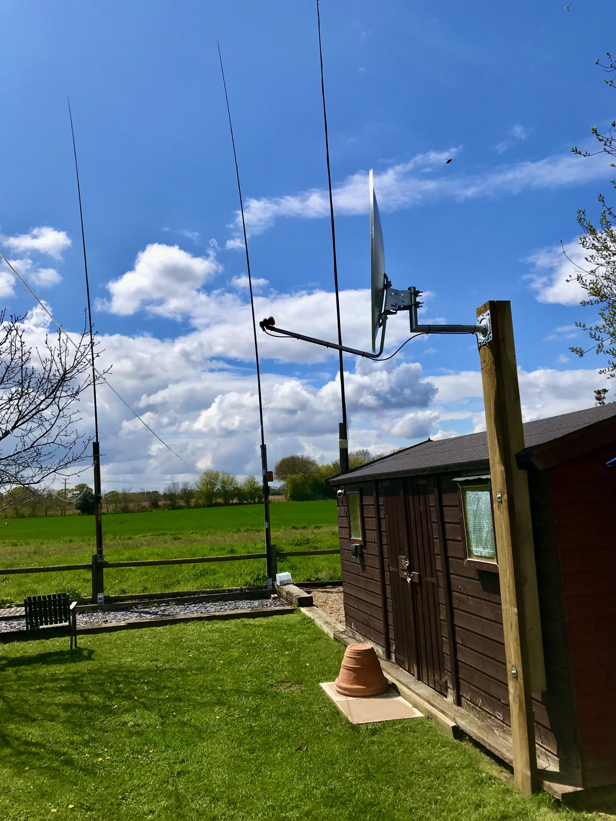
QO-100 dish successfully mounted & aligned with HF antennas in the background
Below is a very short video clip showing a German station talking on the QO-100 satellite. As you can see the signal is nice and strong and extremely clear. I did find that the output from the LNB was actually too much for the FCD SDR and so I reduced the LNA setting in GQRX to 0dB. This reduced the background noise level considerably as the receiver was no longer being overloaded and made the signals much more prevalent above the noise floor.
Short video clip showing signal clarity from the QO-100 Satellite
I’m really pleased at the performance of the receive path and have now ordered the 2.4Ghz hardware from DXPatrol and Nolle Engineering so that I can build the transmit path.
I have also made some improvements to my QO-100 Node Red Dashboard so that I can work split on the satellite using my IC-705 and FCD SDR.
QO-100 Node Red Dashboard with ‘Split’ capability
Once the 2.4Ghz hardware arrives I’ll update the blog with progress.
Following on from my 2m Band Eggbeater Satellite Antenna here’s the design for the 70cm Band version that will enable duplex satellite operation.
The design is basically the same as the 2m antenna but, with smaller dimensions. All modelling has been done with the antenna at 5m AGL.
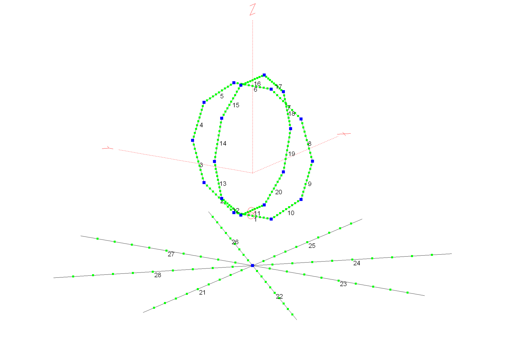
70cm Band Eggbeater Satellite Antenna
Each of the Eggbeater loops has a conductor size of 5mm and a circumference of 73.5cm with the radials exactly 5cm below the bottom of the loops. The 8 radials are exactly 34.15cm long each. The distance between the bottom of the eggbeater loops and the radials must be 5cm to get the best radiation pattern from the antenna.
With these dimensions the antenna has an SWR of <1.5:1 across the whole 70cm band making it ideal for both satellite and general repeater/SSB working.
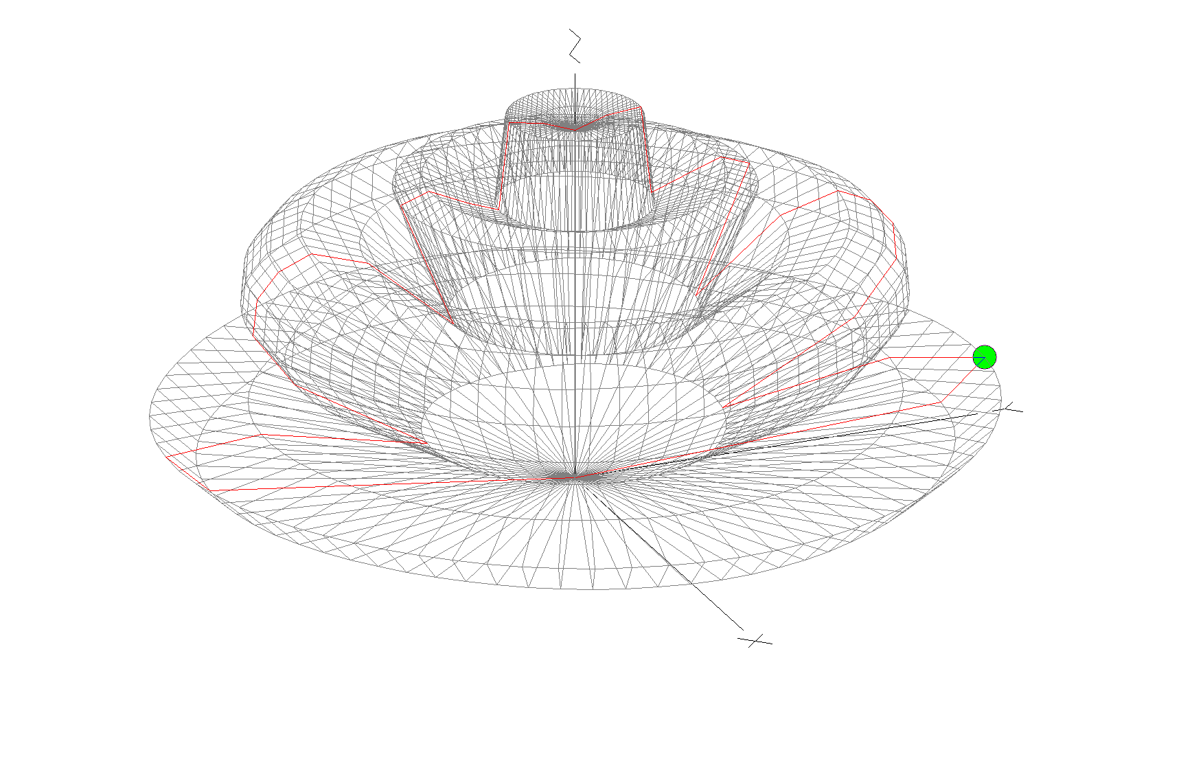
70cm Band Eggbeater Satellite Antenna 3D Far Field Plot
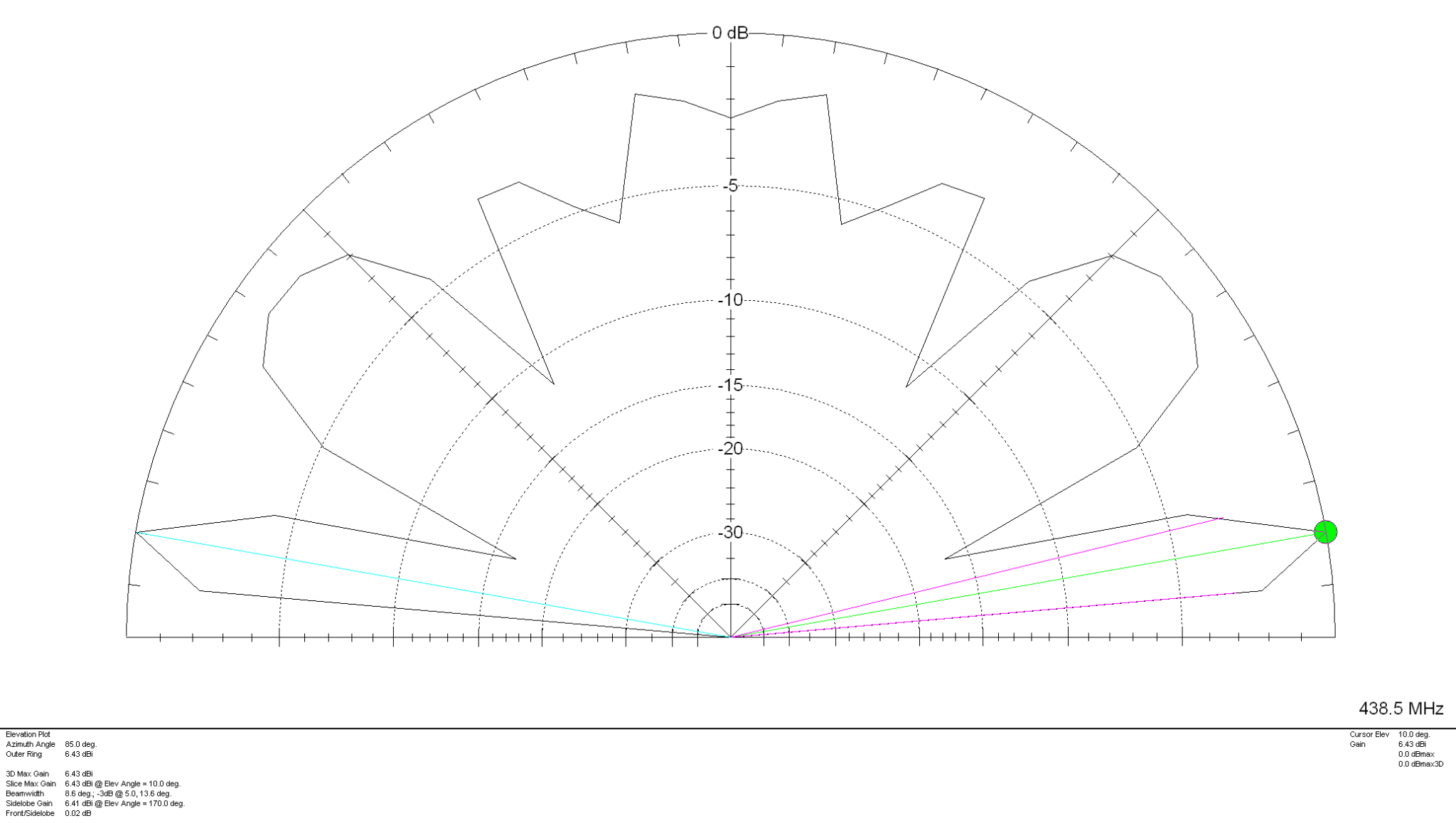
The 3D far field plot shows that the antenna has a good mix of high and low angle radiation that makes it ideal for working satellites at all elevation angles.
70cm Band Eggbeater Satellite Antenna 2D Far Field Plot
The 2D far field plot shows that the antenna has the following high gain lobes:
The null at the top of the antenna isn’t as pronounced as on the 2m model and so this antenna should perform better when the satellite is directly above. Just like on the 2m band version, this antenna must also have a feed phase angle of 90 degrees between the two eggbeater elements. It’s very important that the phasing harness is built accurately as it can impact the radiation pattern of the antenna if the phase angle isn’t correct.
ON6WG has written an excellent article on how to create the phasing harness using 2 pieces of coax cable, this is an ideal solution for this antenna.
I’ve been chatting a lot recently on Matrix about antennas for the amateur satellites.
Since I’m currently working on building a ground station for the QO-100 satellite a group of satellite enthusiasts having been talking about the other satellites that are in orbit around this little planet of ours.
The ISS FM voice repeater on 145.990Mhz is very popular and is one of the easiest satellite stations to get into apparently. Many are using Eggbeater antennas to get an all round radiation pattern.
I’ve never looked into building or modelling such antennas and so I decided to have a go at modelling one and use it as an opportunity to see how it works.
All the modelling has been done with the antenna at 5m above ground level.
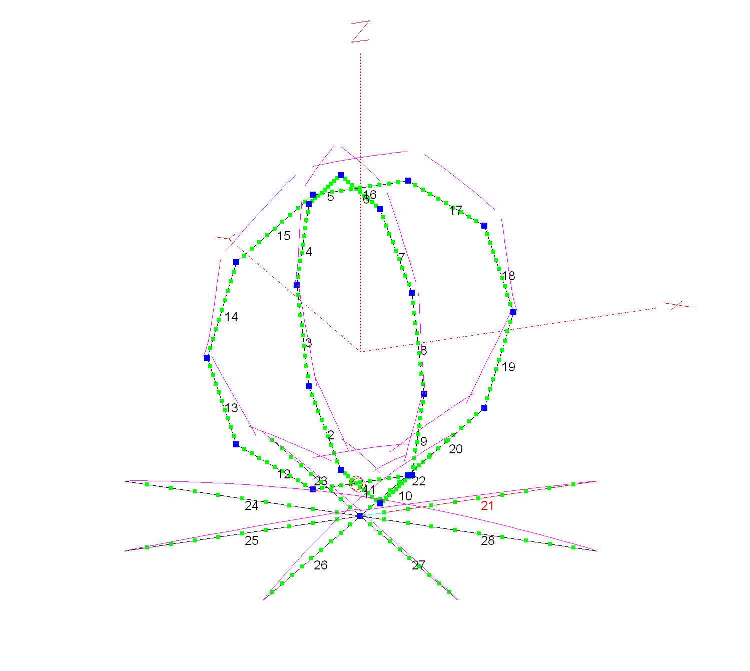
2m Band Eggbeater satellite Antenna with 8 Radials
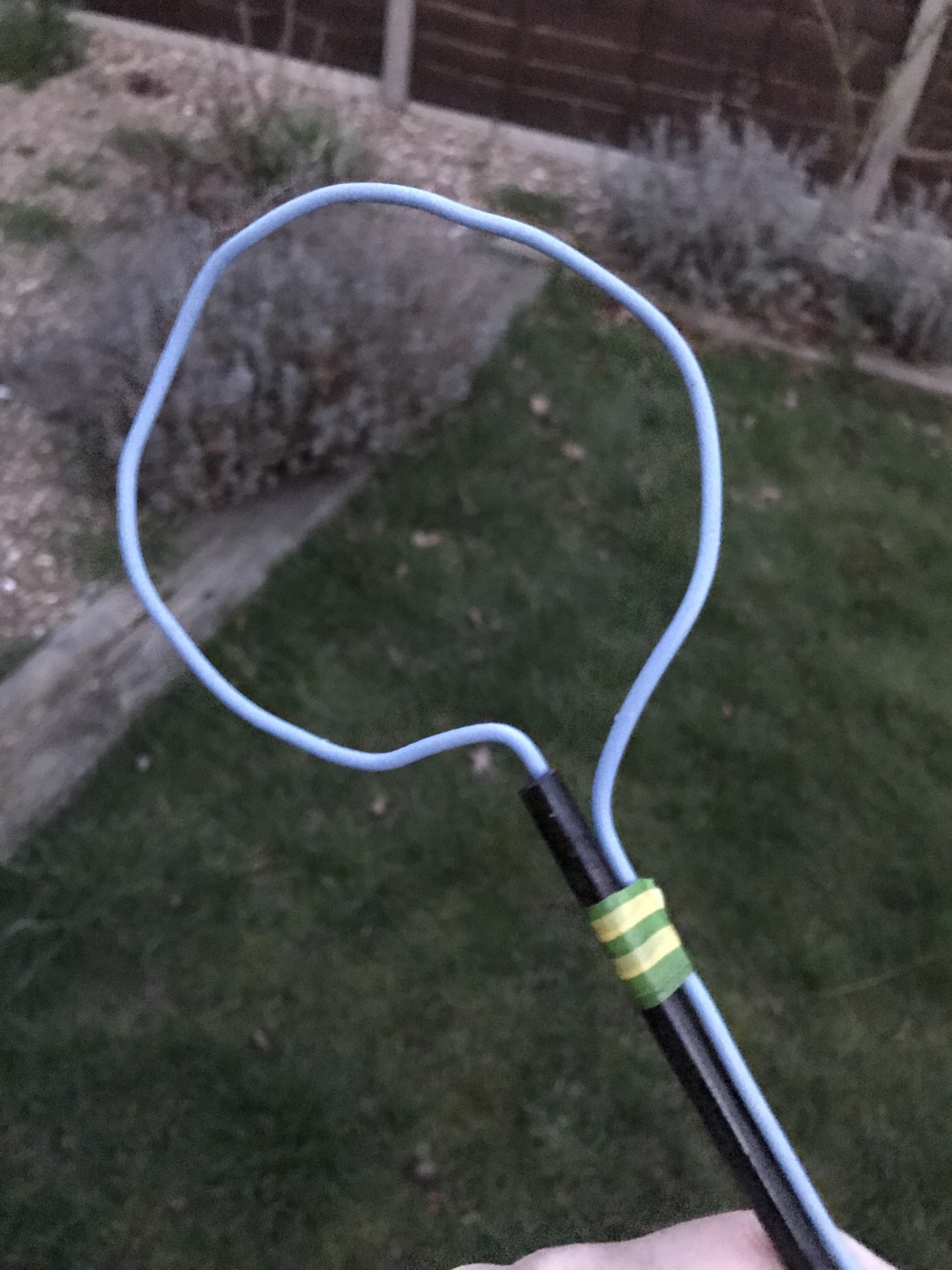
Each loop has a circumference of 2.17m and each of the 8 radials is 0.5425m long and 5cm below the eggbeater elements. I’ve modelled the antenna using 5mm diameter conductors as this should make them resistant to wind etc. I am planning on using 5mm copper tubing for the build.
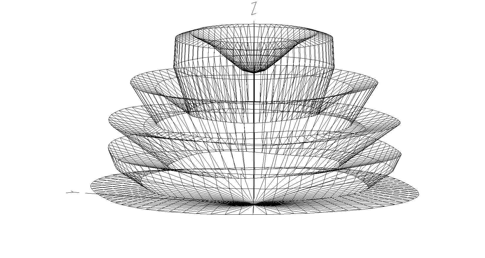
2m Band Eggbeater Satellite Antenna 3D Far Field Plot
The 3D far field plot shows a typical radiation pattern for such an antenna with a very good low angle gain for working satellites on the horizon and multiple high gain lobes as the radiation angle increases. At 5 degrees the RF is horizontally polarised, ideal for shooting directly out at the horizon. This is mainly due to the phasing of the two elements. At the higher angles the RF is vertically polarised thus giving the ability to receive both horizontal, vertical and some circular radiation at a good range of angles. There is however, a very slight null directly above the antenna and so signals to satellites directly above will be attenuated slightly compared to the other two high angle high gain lobes. This will also be the case on receive.
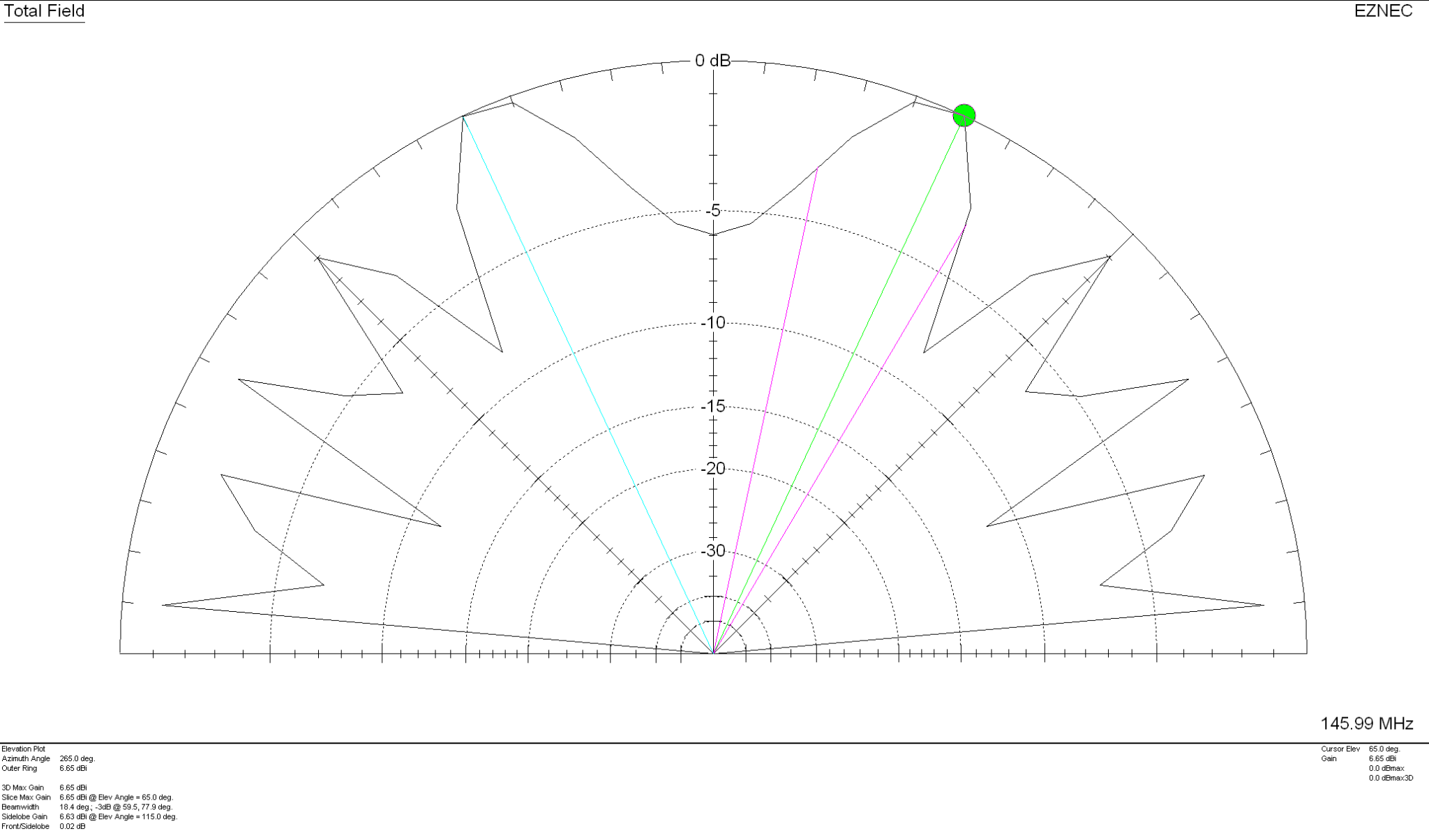
2m Band Eggbeater Satellite Antenna 2D Far Field Elevation Plot
With 5.42dBi gain at 5 Deg this antenna has a real good shot at the horizon with the maximum gain of 6.65dBi being at the much higher angle of 65 Deg. Overall this antenna should work well for all satellites from the horizon up to almost directly above the antenna.
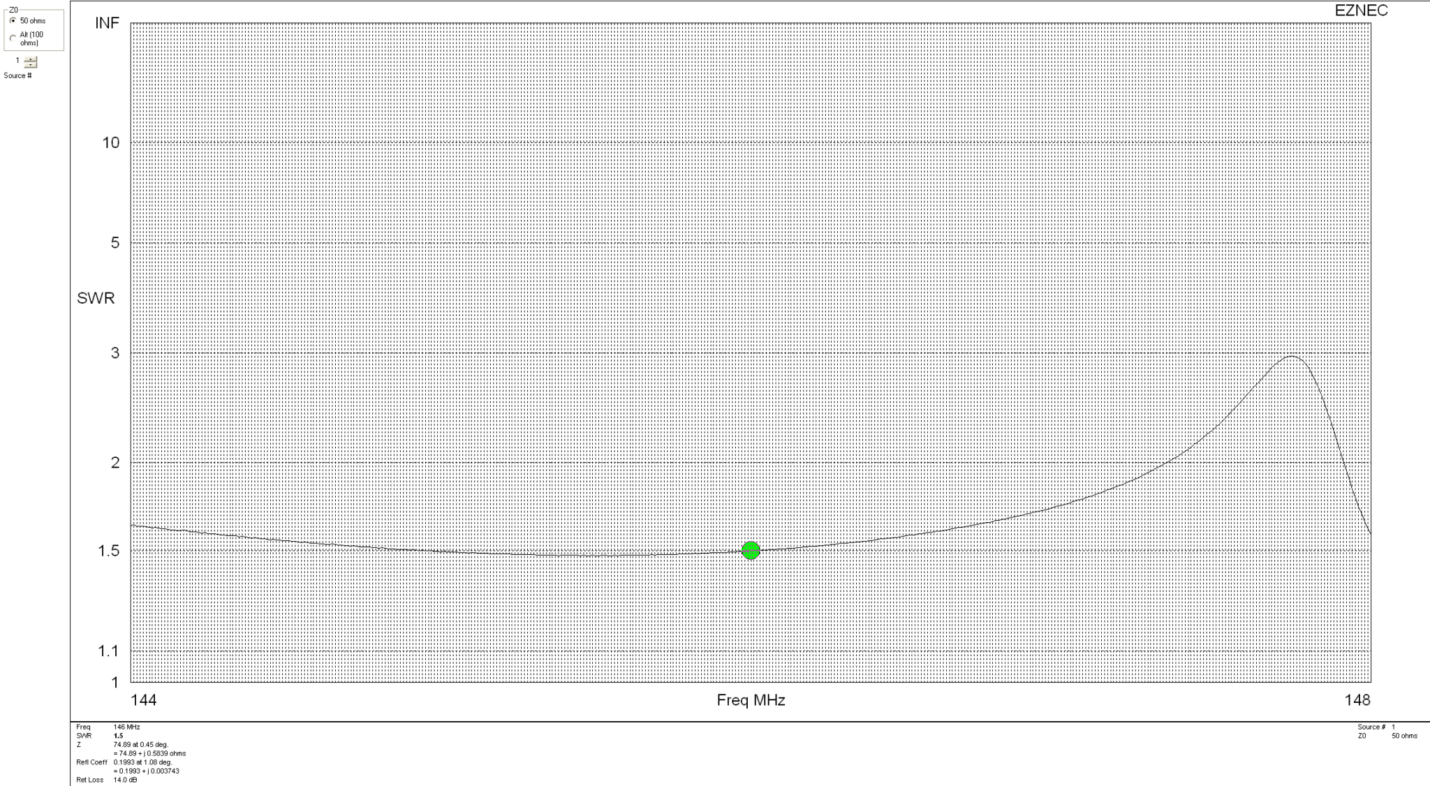
2m Band Eggbeater satellite Antenna SWR Curve
With an SWR of 1.5:1 across most of the 2m band this antenna will match perfectly to 50 Ohm coax feed. It’s really important to remember that when building this antenna the loops must be fed with a phase angle difference of exactly 90 degrees. If this isn’t accurate then the radiation pattern is affected quite drastically and spoils the overall performance of the antenna.
Details on how to create the 90 Degree phase shift between the two elements using 2 pieces of 50 Ohm coax can be found in the excellent article by ON6WG.
Over the years I’ve built many multi band vertical HF antennas including multi-element quarter wave verticals like the DXCommander configuration, multiple end fed vertical dipoles all on the same pole and a host of other configurations. As with all multi band antennas there’s always a compromise, on some bands it performs well and on others it doesn’t, it’s the nature of the beast.
For some time now I’ve been using a multi band vertical antenna that has over the last year performed incredibly well on all bands from 80m to 10m. Don’t get me wrong, it’s not perfect however, it has out performed every other multi band HF vertical I’ve tried to date even though it’s by far the simplest antenna design and according to the antenna modelling software I have it shouldn’t be as good as it is.
So what is this magical multi band HF vertical I speak of? Well it’s nothing more than a piece of wire 13.4m long taped up a 12.4m vertical Spiderpole with 1m of wire tucked down into the top of the Spiderpole.
Obviously this is not going to be resonant on any band without some sort of impedance matching circuit at the bottom of the wire. Originally this antenna was my end fed half wave vertical antenna for the 30m band that was fed via a 49:1 Unun. This antenna worked incredibly well on the 30m band allowing me to work DX globally with ease but, it was a single band antenna and I wanted a multi band solution.
I decided to remove the 49:1 Unun and replace it with a home brew LC circuit made up of a coil made from 5mm copper tubing and a large air spaced variable capacitor I had laying around from an old ATU project I built many moons ago.
This simple LC arrangement at the bottom of the wire worked incredibly well and tuned the wire from 80m to 10m with a perfect SWR on each band using nothing more than a ground rod and 4 x 12m radials. Performance was surprisingly good on all bands 80-10m giving me the ability to get some DX stations that I’ve never been able to hit before. The only drawback to this solution was the fact that I had to go out and manually tune the antenna every time I wanted to change band. Not so much of a problem in the summer but, in the winter in the pouring rain and howling wind it’s no fun at all. (I resolve this issue further down in the article!)
Multi Band Vertical HF Antenna using a 12.4m Heavy duty Spiderpole at the end of the garden
Performance on the HF bands is incredibly impressive with this antenna. Modelling it on EzNEC software it shouldn’t be that great on bands above 20m however, it seems to defy the modelling software as it performs amazingly well on 17m, 15m and 12m, better than any other vertical antenna I’ve made for those bands. How this can be I do not know, normally my antenna builds match closely what the modelling software shows but, in this instance it doesn’t and I’ve really no idea why.
Multi Band Vertical HF Antenna showing loop at top and wire tucked down into pole
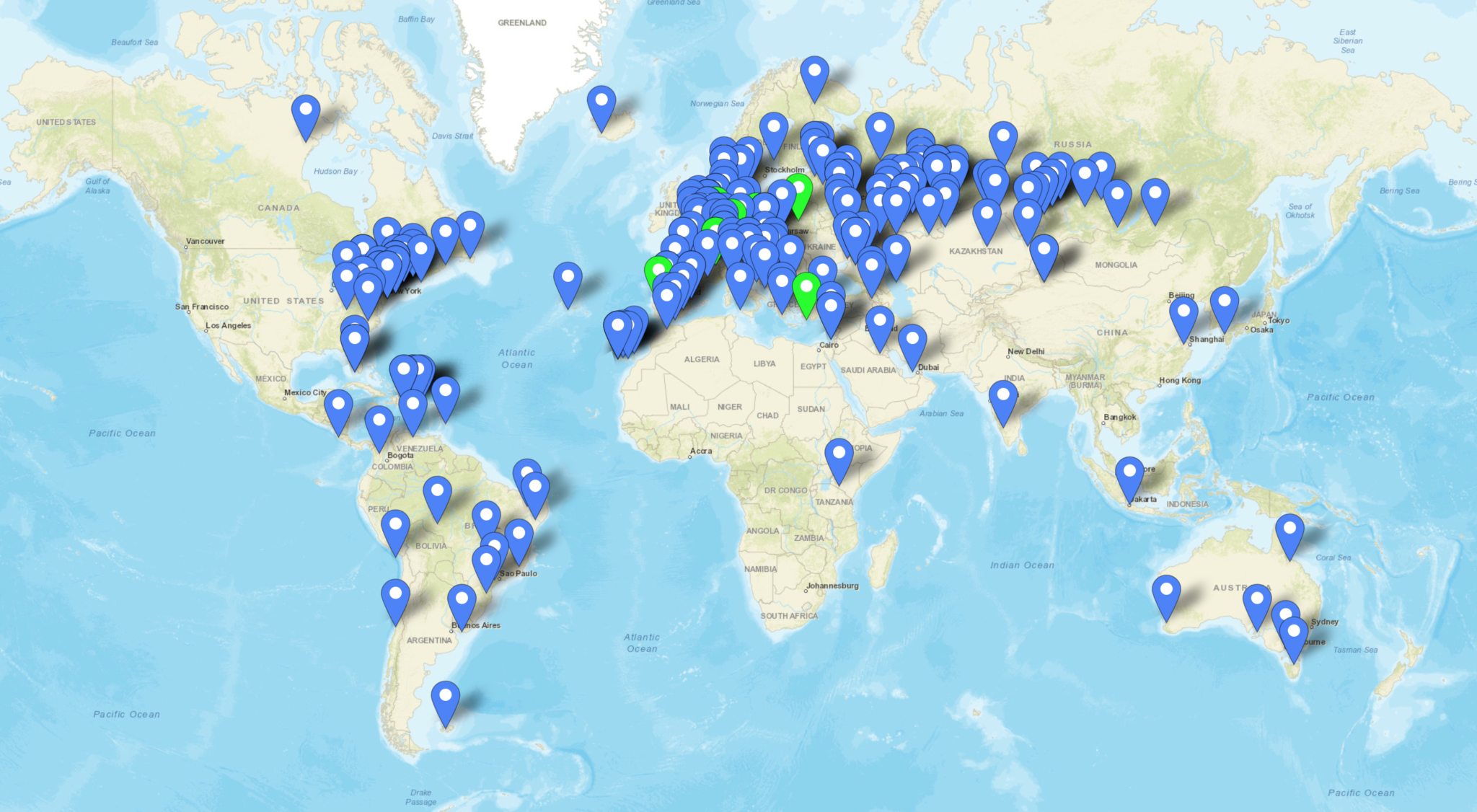
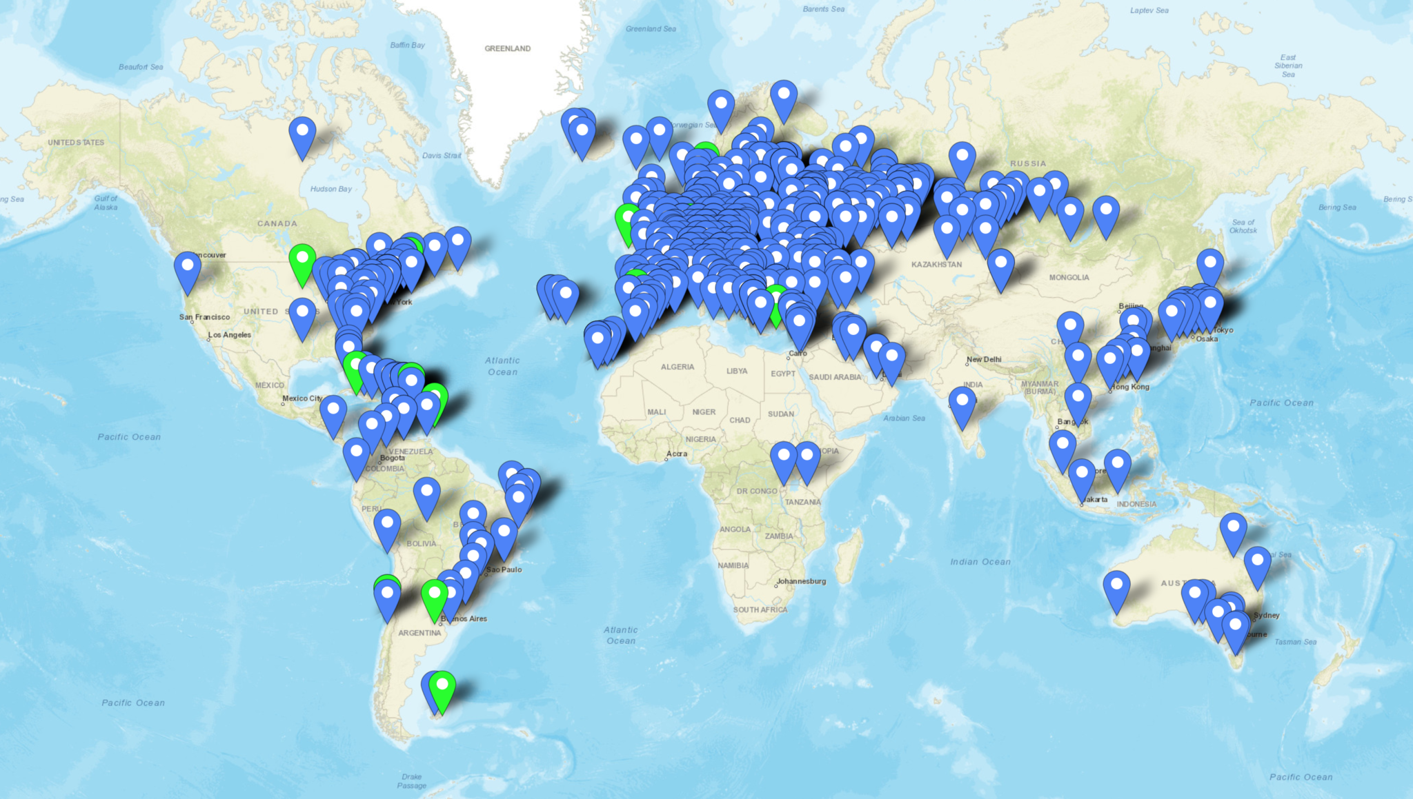
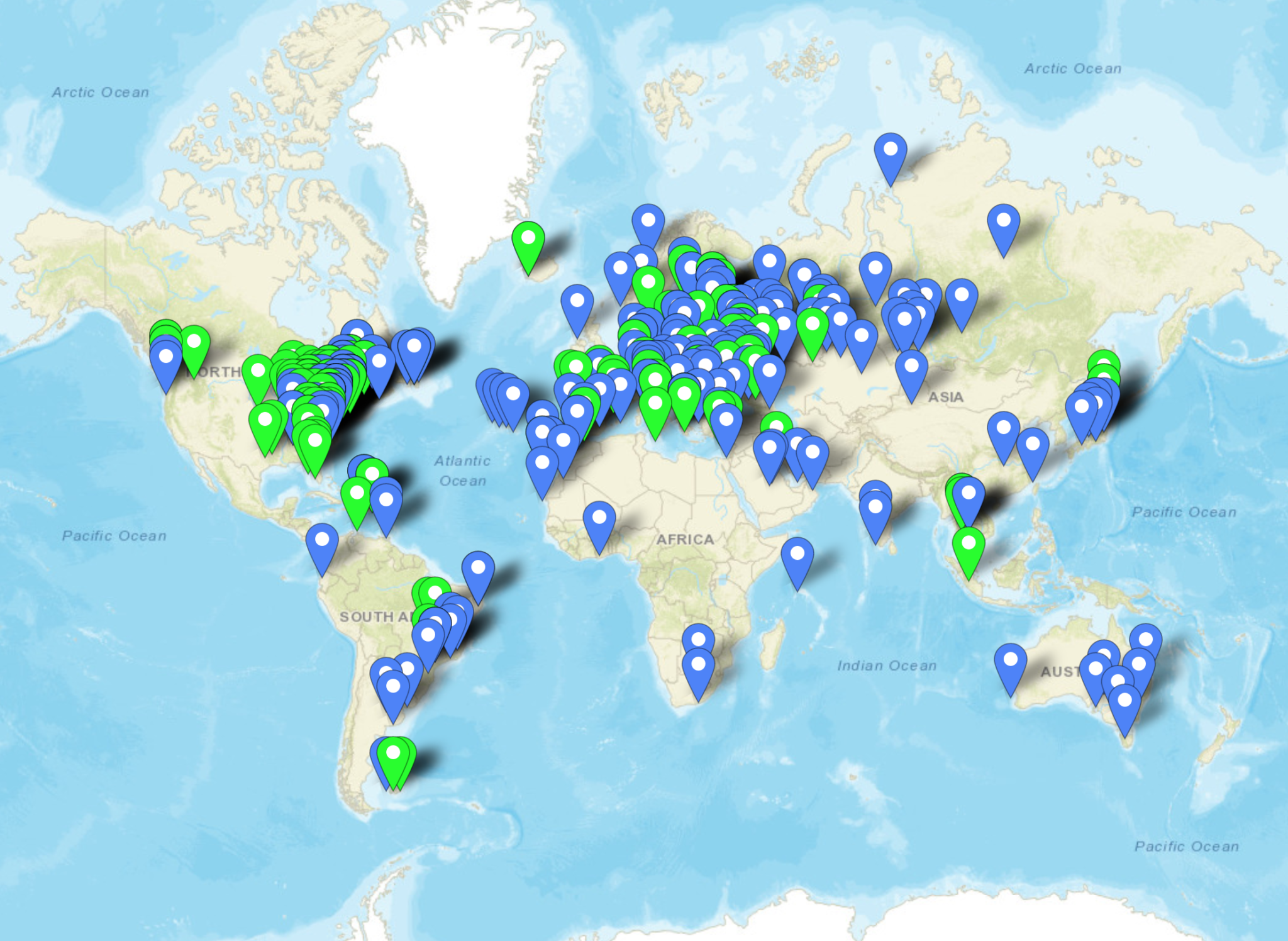
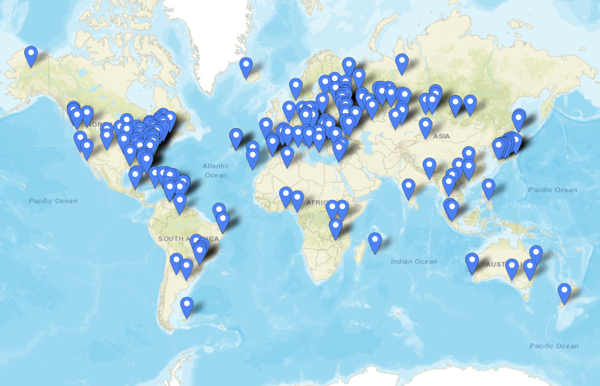
Always wanting to put things into perspective here’s some details of the contacts I’ve made on each band showing how well this antenna has performed over the last year or so.
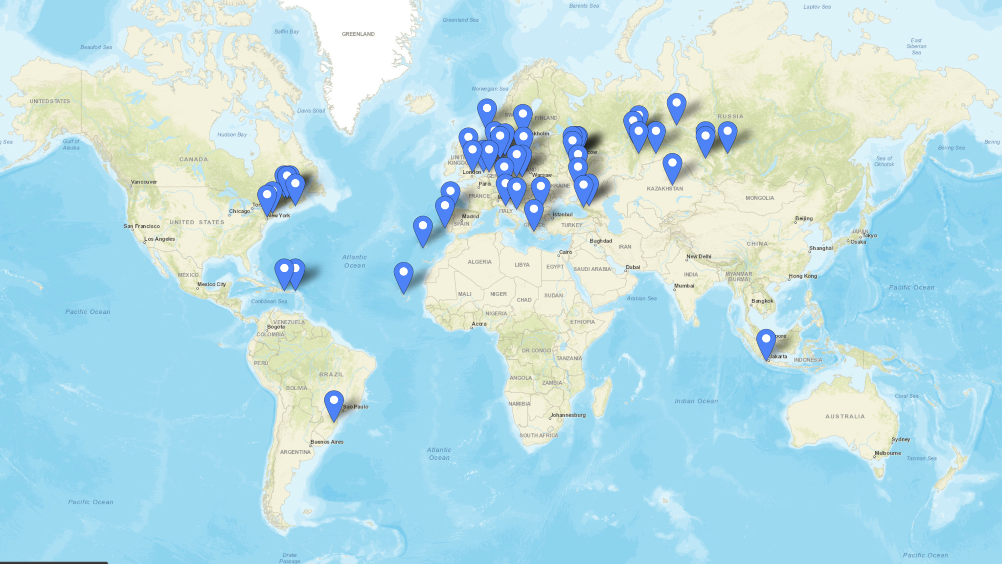
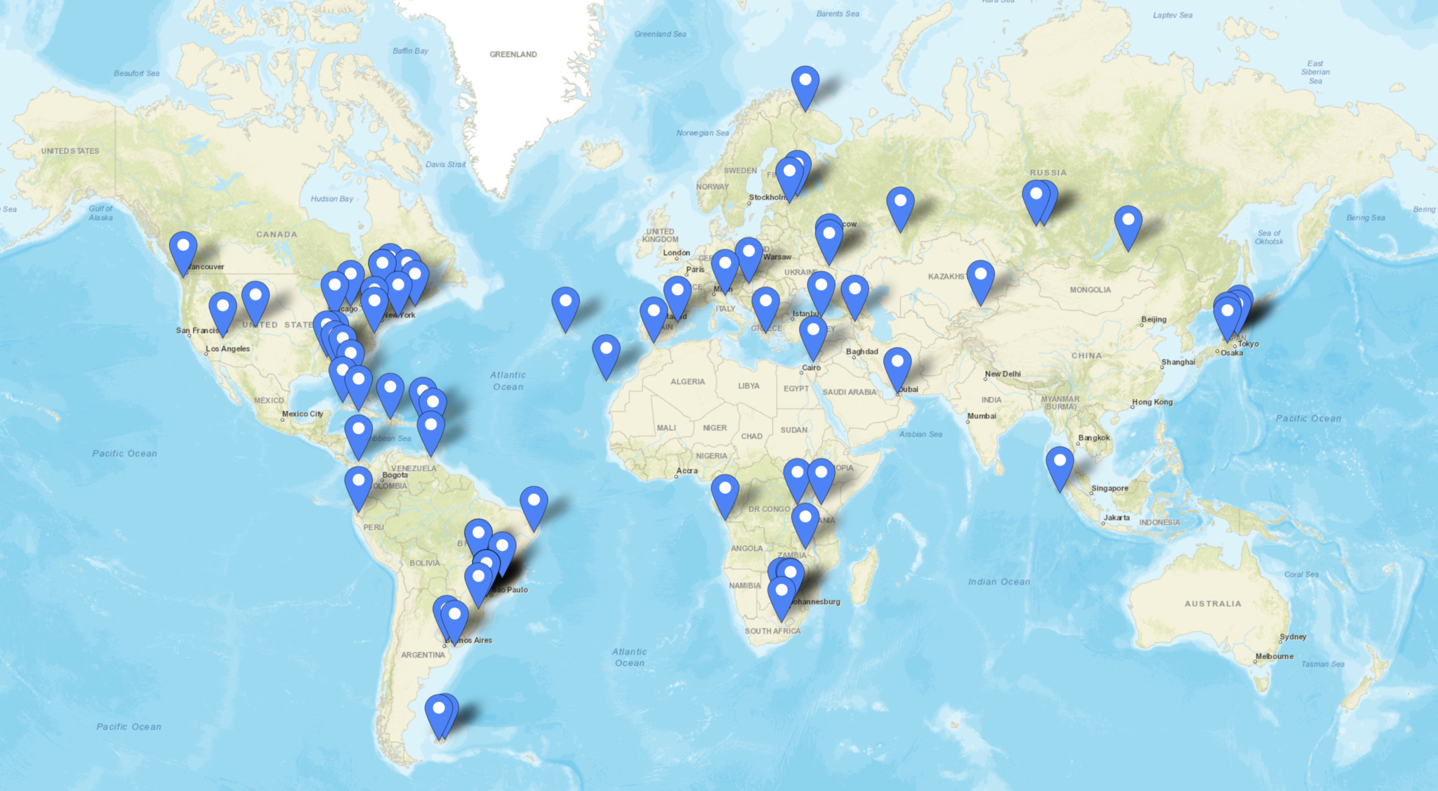
Firstly the 80m band, I’ve not used this band much over the winter months as I’ve got into the higher bands however, the map below shows all the stations worked on 80m using this antenna.
Stations worked on the 80m band from the M0AWS QTH
There are 51 contacts in total, not a big number by any means however, there are some good distances made with contacts into North America, South America and Indonesia. I’m sure I could had done better if I’d spent more time on this band, something to aim for next winter perhaps.
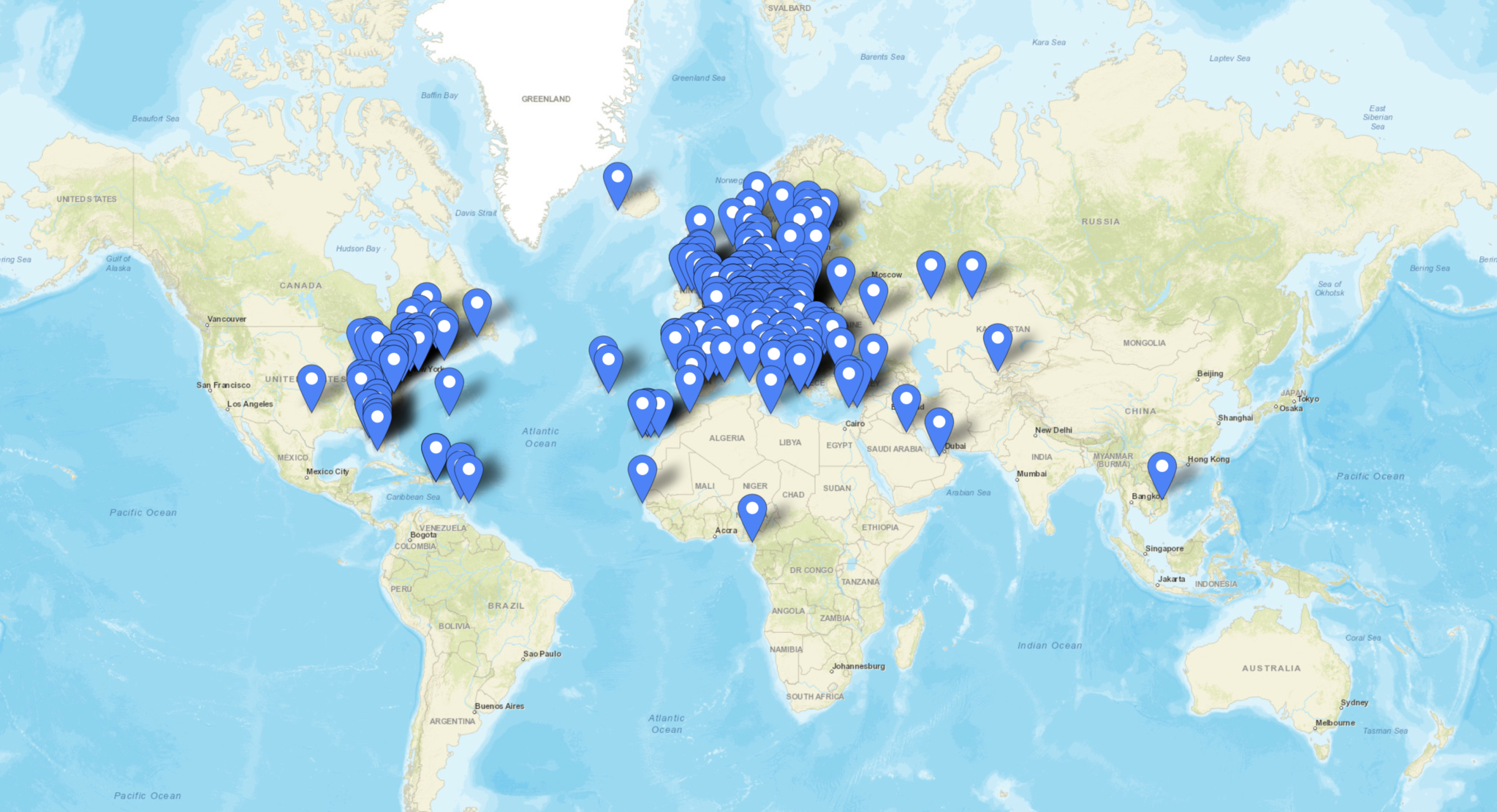
Next is the 60m band, a band I really like and have enjoyed over the winter months. The antenna performs incredibly well on this band even though we have very limited access to 60m here in the UK. With 288 contacts in the log with a good spread of distances I’m really pleased with how this antenna performs on this band.
Stations worked on the 60m band from the M0AWS QTH
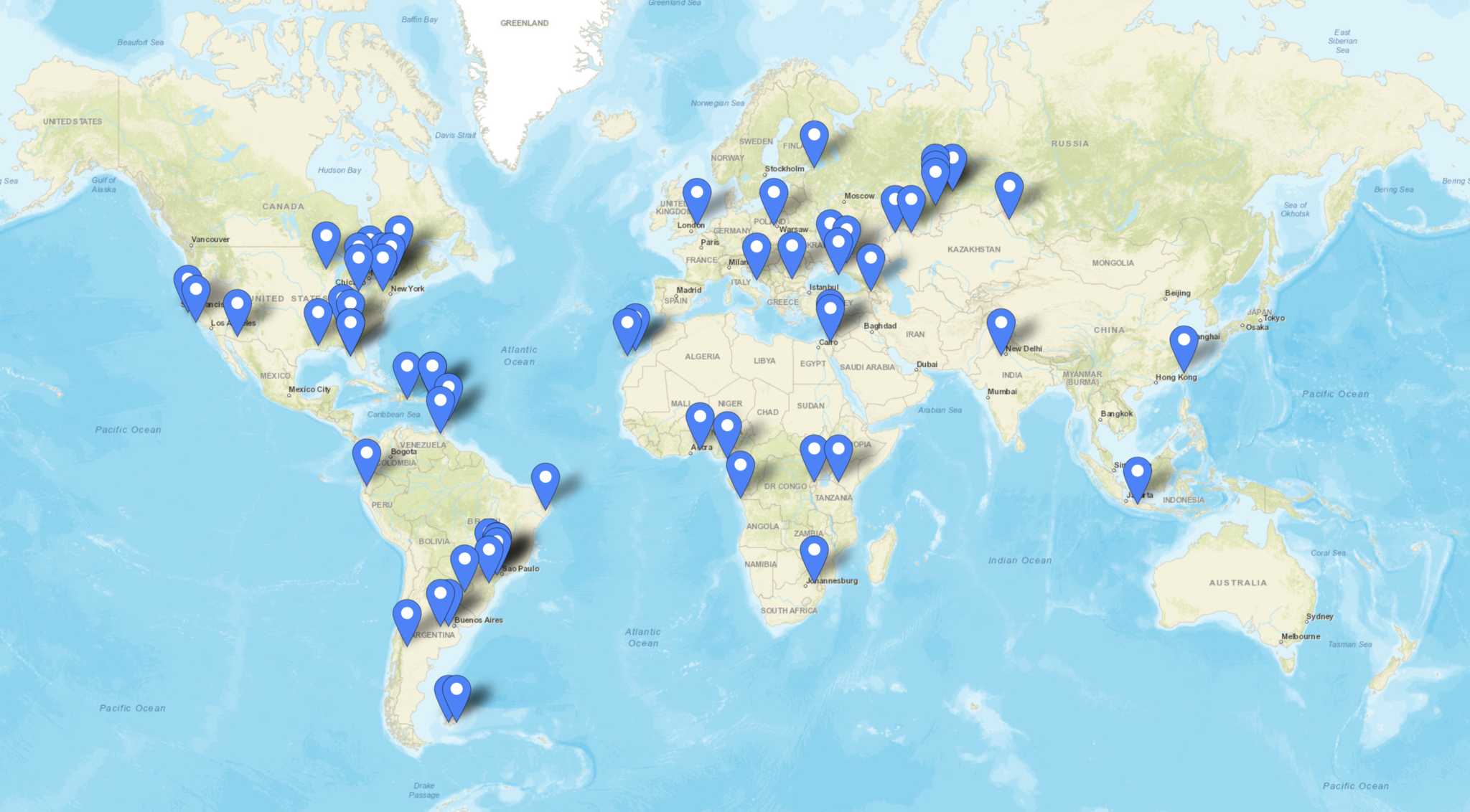
Moving up in frequency the 40m band is the next one on the list, this is a great band and one that I’ve loved for many years. I’ve spent countless hours on CW on this band in the past and worked some great DX. The performance of this antenna on the 40m band is excellent, if I can hear the DX normally I can work them regardless of where in the world they are located. With 226 contacts in the log spread globally over the winter here in the northern hemisphere I have no complaints about performance of this antenna on the 40m band.
Stations worked on the 40m band from the M0AWS QTH
Moving up onto the 30m band I have to admit this is probably my favourite band of all. I’ve spent so many hours on CW working some of the best fists I have ever heard on the air I’ve grown to love this band not just for the DX available but, for the quality of operator found on this narrow piece of the RF spectrum. Needless to say since the antenna is a half wave on the 30m band performance is stunning, out performing any other 30m band antenna I have ever made. It’s even better than the 30m Delta Loop antenna that I built and used when I lived in France.
With 467 contacts in the log on the 30m band you can tell this is my goto band and one that offers access to some of the best DX in the world.
Stations worked on the 30m band from the M0AWS QTH
The 20m band is a band that I never really used until I moved back to the UK from France. Living in France I had acres of land and so I was very much into the low bands, 160m to 30m and never ventured above this part of the spectrum. Now living back in the U.K. with a typical U.K. sized garden the low bands are much more difficult to get onto and so my interests have moved up in frequency somewhat.
Getting onto the 20m band I was amazed at how easy it is to work DX stations compared to the low bands, it’s simply a case of if you can hear them you can work them, there’s no real challenge to be honest. Because of this the band is always super busy with people shouting over the top of each other to get the DX. Not to be put off, I’ve made a surprising 412 contacts on 20m covering the globe. This antenna works incredibly well on this band and you really don’t need anything else to work DX on 20m.
Stations worked on the 20m band from the M0AWS QTH
Next is the 17m band, one of the WARC bands that I’ve never really ventured onto until now. I have to admit I really like this band, when it’s open it’s normally open to the world all at the same time. With an almost undetectable background noise level you can hear the faintest of signal on this band. This is one of the bands that according to the EzNEC modelling software this antenna shouldn’t be any good on but, I have to say that it’s performance is beyond anything I ever imagined. I’ve worked my longest distance yet on this band and with this antenna, ZL4AS at 11776 miles, a distance I haven’t achieved yet on any other band. The 17m band really is a great band, I’d actually say it’s better than the 20m band even though there is considerably less spectrum available. With 220 contacts in the log it’s been a fun band to use.
Stations worked on the 17m band from the M0AWS QTH
Continuing the theme of the WARC bands, the 15m band is another one that I’ve only discovered in the last 12 months. It’s only now that I realise what I’ve missed out on due to my addiction to the low bands for so many years.
I’ve only made 76 contacts on the 15m band, not a lot at all really. This is mainly due to the fact that I get easily side tracked by the 17m and 30m bands most of the time and the radio VFO never gets as far as 21Mhz. Performance of the antenna is good on 15m, I would say not as good as on the 17m band but, it’s no slouch by any means.
As you can see on the map below, I may of only made 76 contacts on the 15m band but, they are spread right across the world proving that this antenna’s DX-ability on 21Mhz really is rather good.
Stations worked on the 15m band from the M0AWS QTH
Finally we arrive at the top of the WARC bands, the little 12m band. Once again this band is very much like the 17m band, super low background noise level, when it’s open you can work huge distances with very little power but, often there is quite deep QSB that can make getting that elusive DX a bit more challenging.
With only 66 contacts in the log once again I’ve not spent a huge amount of time on this band but, it hasn’t disappointed. With global coverage from this antenna on 12m once again I am astounded at how well it works. With software modelling saying it should be terrible on 24.9Mhz with nothing but super high angle radiation, it really shouldn’t be a good antenna for DXing on this upper WARC band but, it is and I have no idea as to why!
Stations worked on the 12m band from the M0AWS QTH
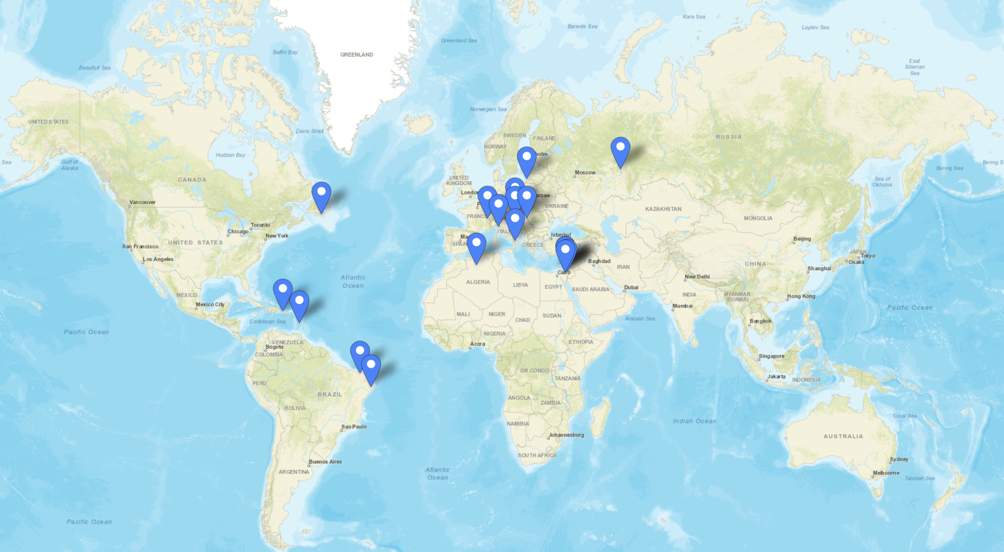
Finally we arrive at the 10m band, another band that I have never got into even though many refer to it as the magic band. This is the band that I’ve made the fewest contacts on, not because the antenna doesn’t work at the dizzy heights of 28Mhz but, because I hardly ever get the VFO dial past the lower bands due to the level of DX available. I really should make more effort to get the best out of the 10m band, especially now the summer is coming.
With a measly 19 contacts in the log I should be ashamed of myself for not doing more on this band as it is very often open and busy with traffic. Since I’ve not really used the antenna that much on the 10m band it’s hard to say how well it performs however, I have had contacts into North and South America and so it shows potential.
Stations worked on the 10m band from the M0AWS QTH
As you can see, the performance of this antenna is self evident from the log entries, it works superbly even though the modelling software says it shouldn’t above 14Mhz. This is now my main antenna here in the U.K. and I’ve only made one change to the initial setup and that is to add a CG3000 remote auto ATU to replace the home-brew LC tuning circuit.
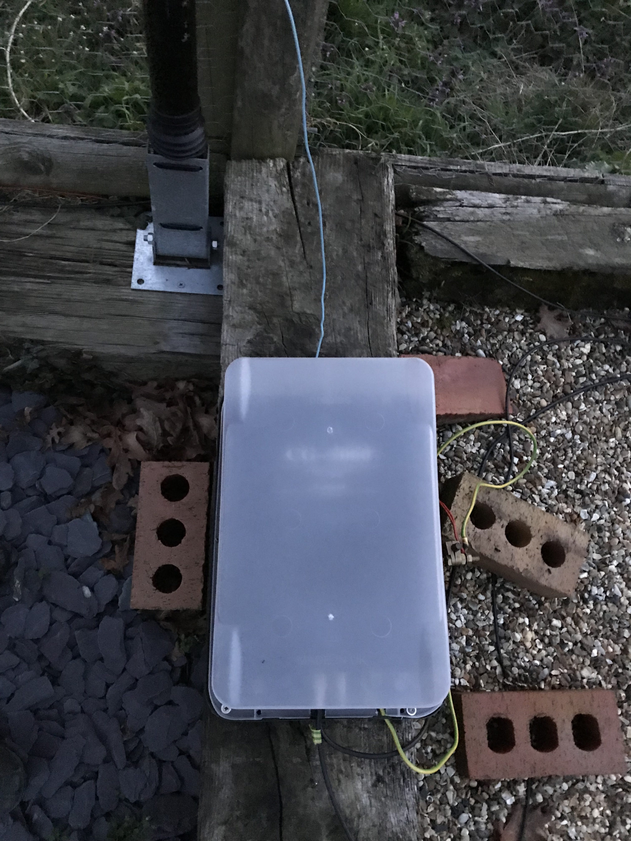
CG3000 Remote Auto ATU housed in a plastic box
With the CG3000 auto ATU in place I no longer have to venture out into the cold, wet garden in the winter months to change band, it’s just a case of sending a continuous 10w signal into it and leaving it to tune in less than 2 seconds. The CG3000 is a Pi Network ATU so it handles both high and low impedance loads with ease. A Pi Network ATU is one of the best you can have, I’ve made my own in the past and had excellent results.
So in summary, 13.4m of wire vertically up a 12.4m pole with 4 x 12m radials, a ground rod and a CG3000 Auto ATU will give any HAM station the ability to work DX on all bands from 80m to 10m without ever having to leave the shack to tune it.
Since I got the CG3000 off of Ebay for a bargain £170 and the 12m heavy duty Spiderpole for under £100 the total cost of the antenna is considerably less than many commercial offerings available and yet performs as well if not better.
If you want to get this antenna onto the 160m band then you just need to add a small coil into the mix at the bottom of the wire to increase the inductance in circuit. The CG3000 will then happily tune the entire 160m band. It’s best to remove this coil though for all the other bands otherwise performance is reduced.
Please be aware that the performance of this antenna will not be anywhere near as good if you use the ATU in your radio at the end of a coax run. This is because the coax becomes part of the antenna and the radiation pattern is all but destroyed. You will be extremely disappointed if you use the antenna in this fashion. The ATU must be at the end of the wire and connected directly to ground and the radials to get the performance that I have experienced.
Finally, if you have an Icom IC-705 and AH-705 remote auto ATU you can use the AH-705 ATU in place of the CG3000, you will get the same results as I have with the CG3000.
I have used my AH-705/IC-705 combo quite a few times with this antenna with excellent results although, the big antenna can sometimes result in the receiver of the IC-705 getting overloaded especially on the lower bands. This is easily resolved by reducing the RF Gain on the radio.
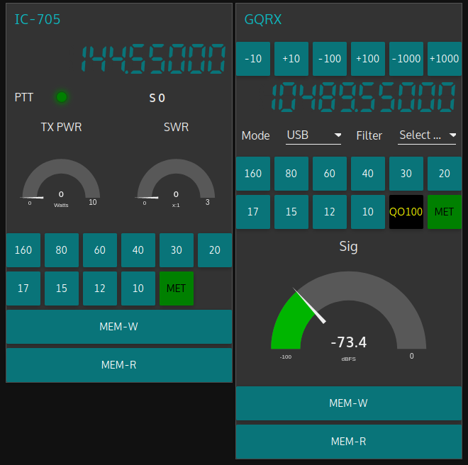
I’ve now completed the GQRX Receive and Icom IC-705 Transmit dashboard in Node Red. It was a fun project to put together and needed some javascript coding to get the functionality I wanted but, I got there in the end.
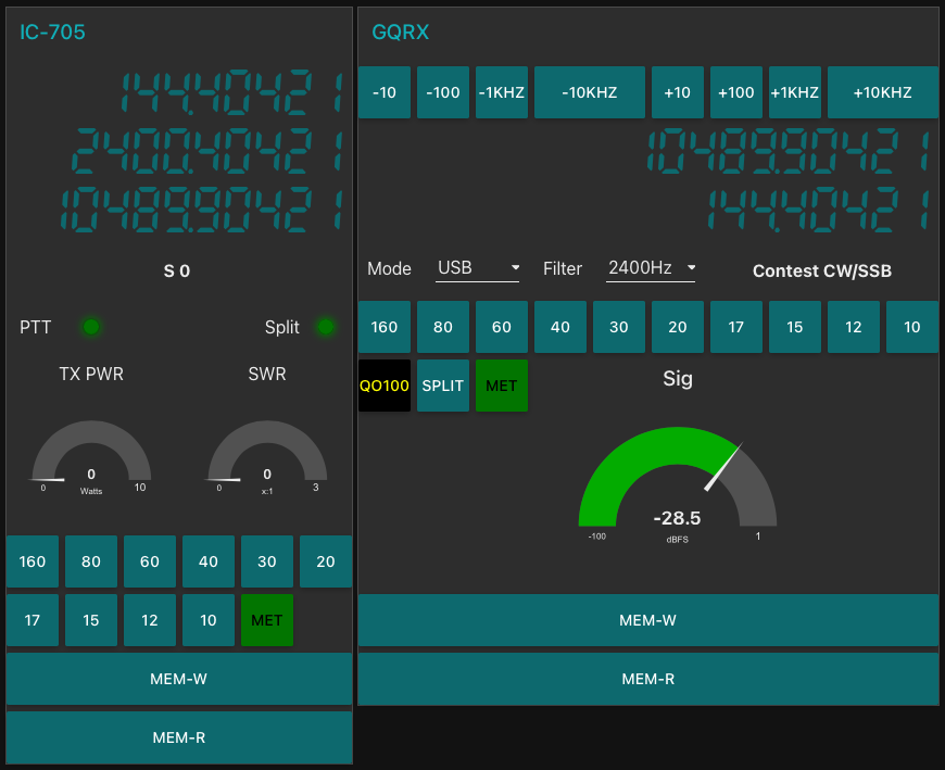
M0AWS QO-100 GQRX/IC-705 control dashboard
The dashboard looks fairly simple but, there is a lot behind the scenes to get it to this stage.
On the left is the Icom IC-705 transmit control panel. It shows the transmit frequency, power output and SWR reading. The SWR is so that I can check that the input into the 2.4Ghz transverter doesn’t have any connectivity issues. The “S0” will actually display the S Meter reading when the IC-705 is being used as a normal transceiver rather than being in QO-100 Duplex mode as shown above where the GQRX app and Funcube Dongle SDR are being used as the receiver.
The GQRX side of the dashboard shows the downlink frequency which tracks the uplink frequency of the VFO on the IC-705. This will ensure that the Funcube Dongle Pro+ SDR receiver will always be on the correct downlink frequency relative to the uplink frequency, thus I should always be able to hear my own signal coming from the QO-100 satellite.
Once taken out of QO-100 mode the two radios can be used independently on any of the HAM bands and can be switched using the buttons on the dashboard.
I also coded in a simple memory facility where a frequency can be stored in Node Red and recalled later on both the transmit and receive sides.
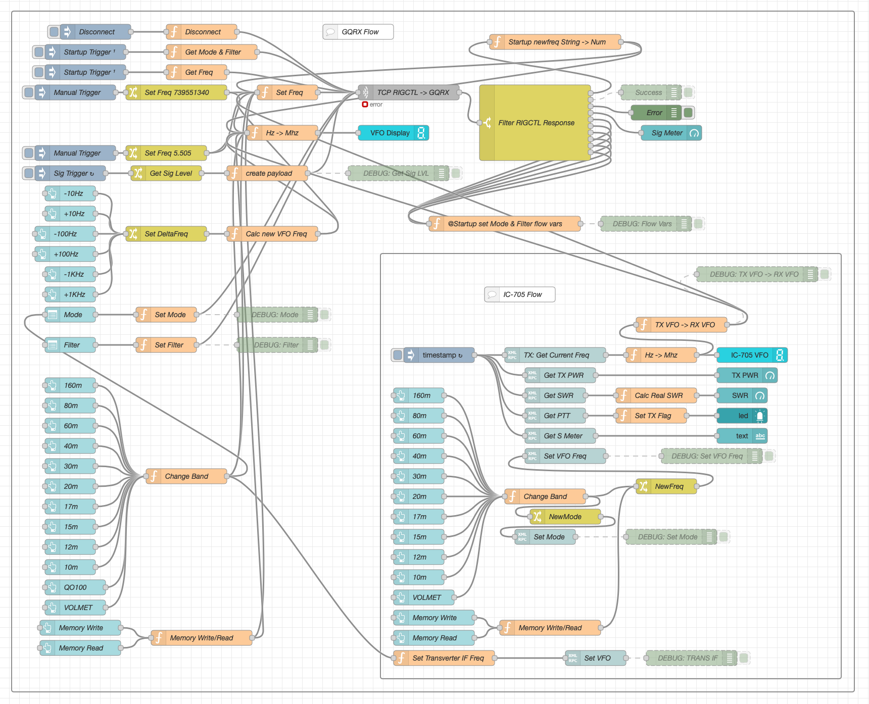
Looking at the dashboard it all looks simple and straight forward however, if you look at the Node Red flow it becomes obvious that this isn’t the case.
QO-100 Dashboard Flow in the Node Red Editor (Click for larger image)
There’s a lot to the flow to get the information from the receiver and transmitter so that it can be presented on the dashboard. There’s also some code to convert between Rigctl protocol used by the GQRX application and XMLRPC used by the IC-705 via FLRig and WFview. I had to also code around a bug in the Node Red XMLRPC node whereby you have to add 0.1 onto the VFO frequency for it to be passed onto the radio otherwise the information is never sent. This was a real pain of a bug to find but, with a little experimentation I found the problem and managed to code around it. The strange thing about this is that the 0.1 added onto the frequency isn’t actually passed onto the radio via the XMLRPC node, it just has to have that on input otherwise it doesn’t work at all. A very strange bug and hopefully one that will be fixed by the node developer in future releases.
All that is left to do now is add the temperature sensors dashboard to complete the dashboard. These haven’t arrived yet and so I’ve not been able to create the necessary flow to collect the data from them.
Hopefully this coming week the weather will improve and I’ll start getting the dish antenna up and the get the receive side working.
UPDATE: Further development of my QO-100 Dashboard has taken place, you can read all about it here.
Whilst I’ve been waiting for the weather to improve so that I can get my QO-100 dish antenna up I’ve been working on my QO-100 Node Red dashboard.
The idea of the dash board is to bring together the operating of the receiver and transmitter into one control centre so that the two separate devices are able to communicate and behave as if they were actually one device, like a transceiver rather than being individual components.
Ideally I would like to have the transmitter and receiver talking to each other such that when the VFO on the transmitter is incremented/decremented the receiver VFO also moves by the same amount.
By doing this the receiver VFO should always be in the right place on the 10Ghz band to hear my 2.4Ghz uplink signal and of course, any station coming back to my CQ calls.
So far I’ve only been working on the receive part of the Node Red flow, it’s certainly been a lot of fun getting it put together.
I control my Funcube Dongle Pro+ (FCD) using GQRX SDR on my Kubuntu PC. This software is working extremely well with the FCD and I’m happy with the level of functionality it offers.
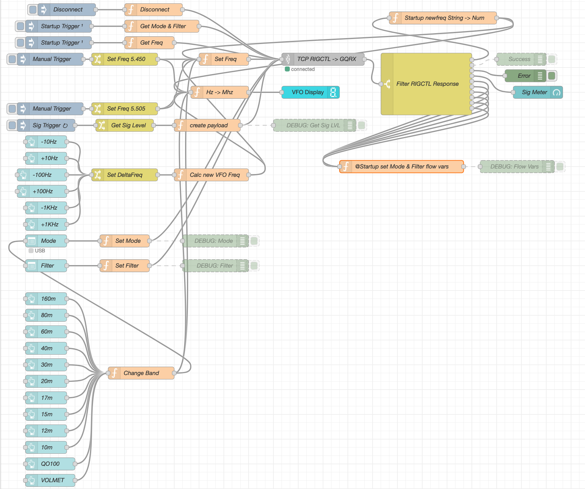
GQRX SDR has the ability built in to control the SDR via remote TCP connection using RIGCTL protocol. Currently there isn’t a RIGCTL node available for Node Red so I have written a number of Javascript function nodes that provide the appropriate functionality in conjunction with a standard Node Red TCP node. This is working extremely well on the local LAN in the radio room and is proving to be very stable and responsive.
M0AWS QO-100 Node Red Flow – Receive Section
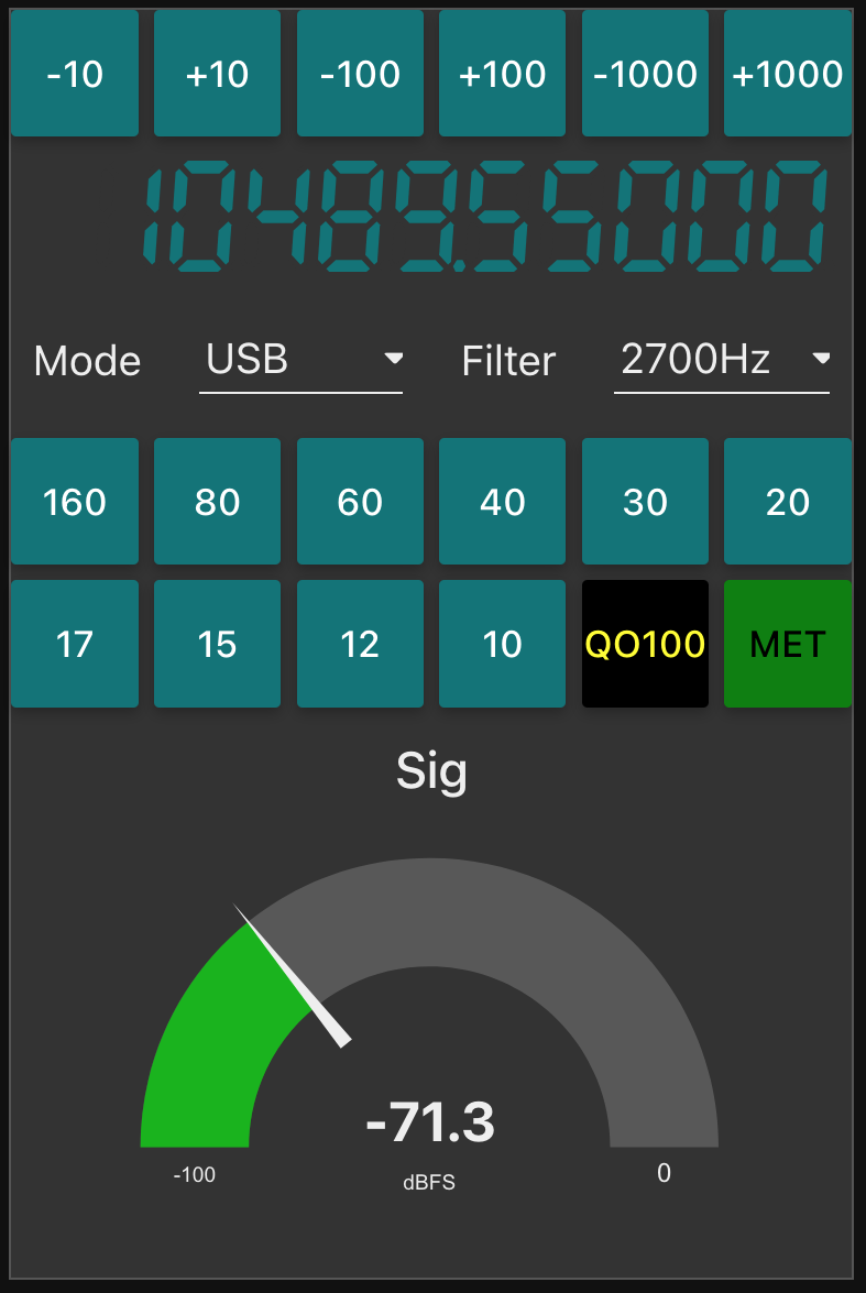
The flow for the receive section of the dashboard looks fairly complicated but, in reality it’s really not too difficult to get to grips with. The receive flow provides the facility to switch bands, switch modes, change receiver filter band width, display a realtime signal strength meter, receive +/- clarifier in 10/100/1000Hz increments and put the receiver into QO-100 mode where the SDR VFO is tuned to 739.550Mhz whilst the dashboard VFO shows the QO-100 downlink frequency in the 10Ghz band. This is all working very well and I’m happy with the initial result.
M0AWS QO-100 Receive Dashboard in QO-100 mode
I now need to start work on the transmit side of the QO-100 dashboard and get communications between my IC-705 transceiver and the FCD SDR working via Node Red. This could be a little more challenging as it will involve communicating with the IC-705 via WFView over wifi.
Following on from my initial article on plotting realtime WSJT-X decodes on a Node Red map I’ve made a few enhancements to the flow so that it includes even more data then before.
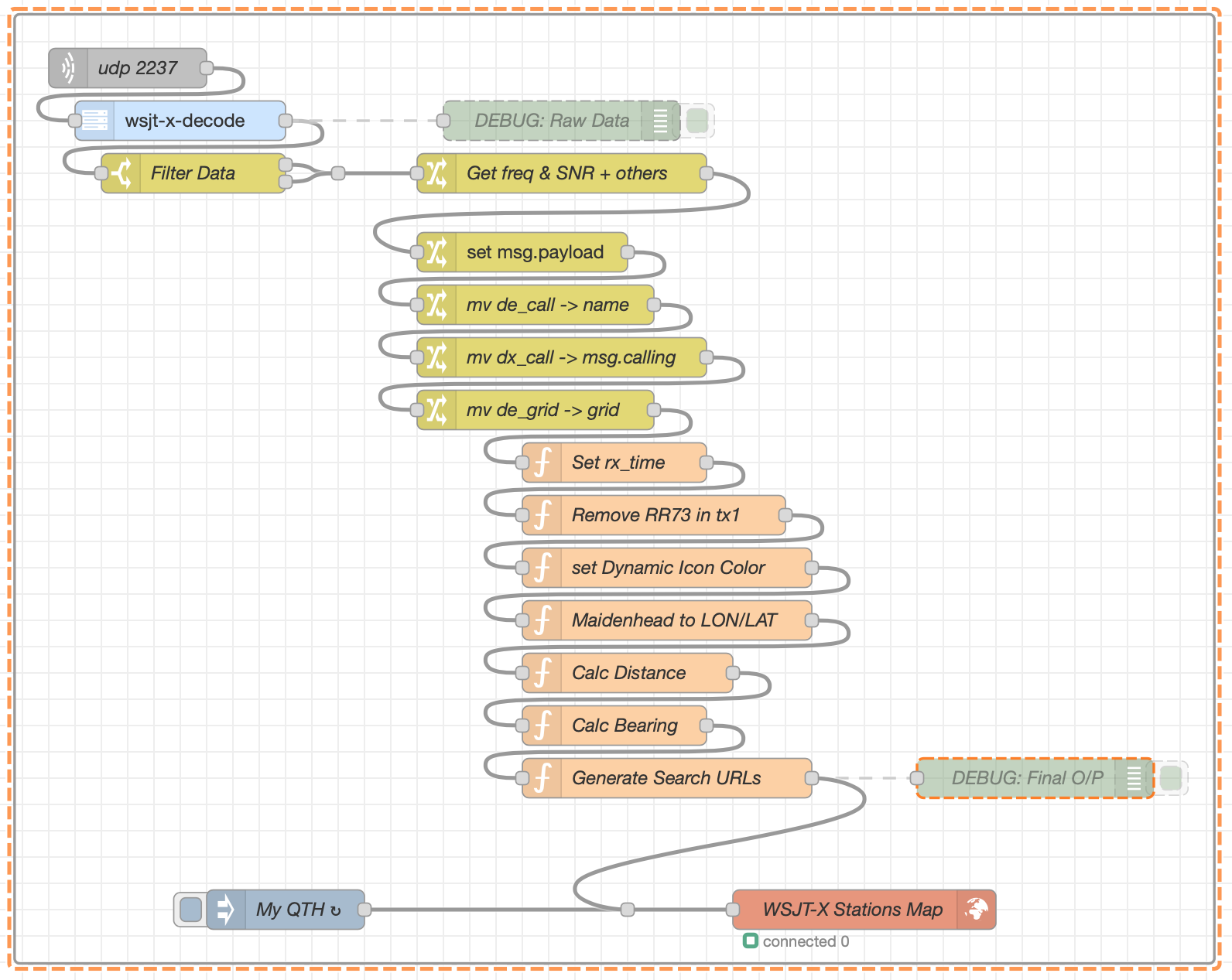
The additions to the flow now enables collection of status information from WSJT-X so that the flow is able to capture the frequency that the radio is tuned to and also the mode that WSJT-X set to. Neither of these two bits of data are in the decode message payload and so a separate mini-flow has to be created to collect the data from the status payload along side the other main flow.
Node Red flow showing additional sub flow in the top left corner of the flow editor screen
Since the status information needs to be available to all other flows I used flow variables to store the status information in so that it can be addressed directly from any of the other flows in the Node Red app.
If you’d like to use the flow in your radio room then I have put a download link below for a file that you can import into Node Red and build the flow in an instant.
Following on from my other Node Red exploits I’ve put together a flow that creates an interactive map of contacts that is generated from the WSJT-X ADI log file.
The flow is fairly straight forward and self explanatory so I won’t go into detail here but, will make a copy of the flow available for download at the end of this article.
Node Red Flow for processing the WSJT-X ADI Log file
The flow is incredibly quick at generating the map with all the pins on it, one for each station worked. The pins are colour coded, blue for FT8 and green for FT4. If you want to add other modes then just create a new colour entry in the Dynamic Icon Colour function.
The resultant map is fully interactive with each pin being clickable showing the QSO information in a tiny popup.
Node Red map generated from the WSJT-X ADI Log file
You can download the flow and try it yourself using the link below.
Following on from my previous article on Enhancing Digital modes with Node Red I’ve now got to a point where I have realtime decode information from the WSJT-X digital application being plotted on a Node Redworld map not just for CQ calls but, for stations in conversation too.
The flow has become somewhat more complex than it was originally as more and more functionality has been added. I have deliberately split out the flow process into more nodes than are really necessary so that the flow is easier to understand. Anyone from a programming background like myself will soon realise that a lot of the nodes could actually be combined into one big node however, the overall flow process wouldn’t be so easy to understand for the Node Red newcomer and would possibly put people off from trying it out.
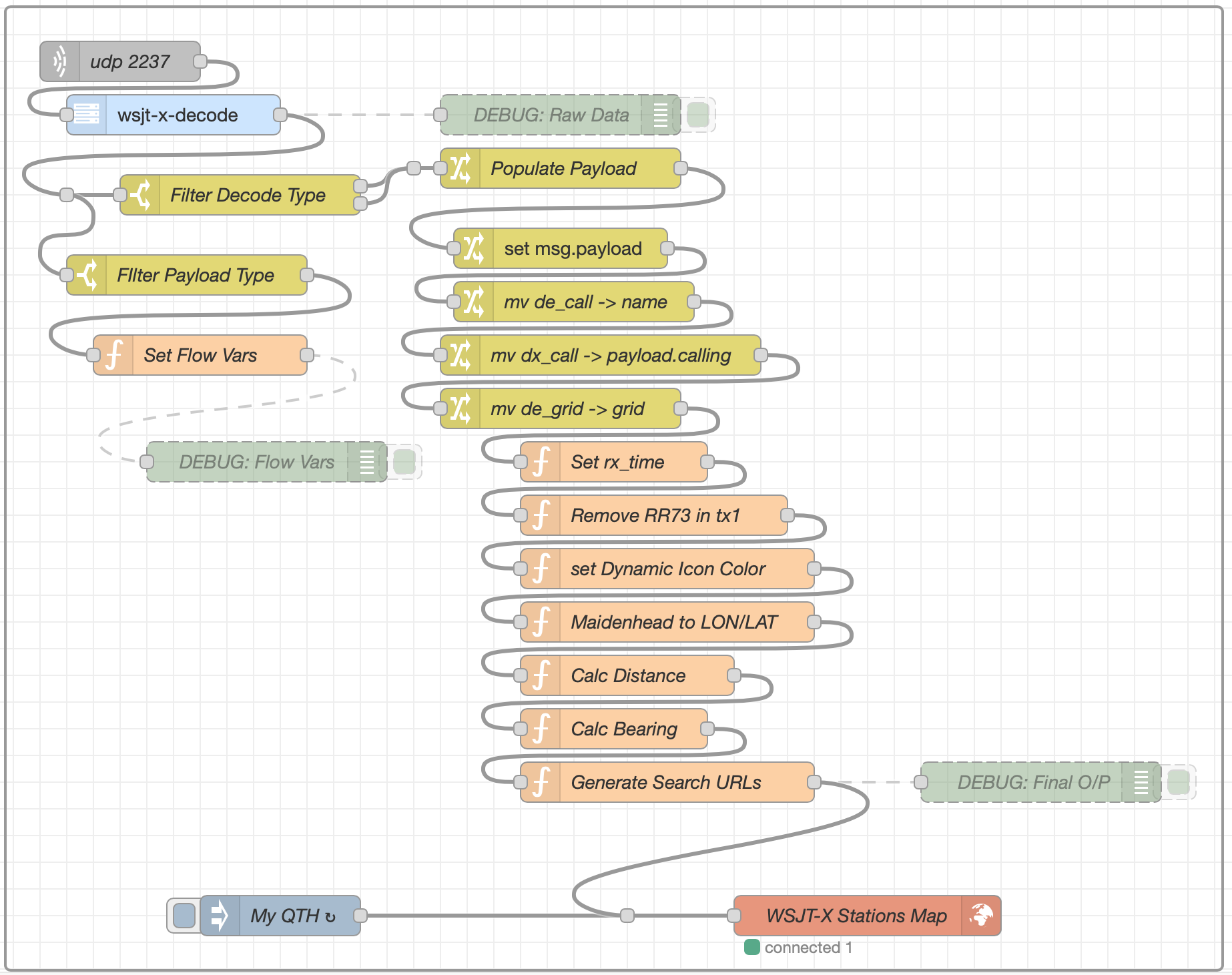
Current WSJT-X Node Red flow
Above is a screenshot of the flow as it currently stands. It’s pretty easy to understand what is happening in the flow due to the fact that the processes are broken out into small, easy to digest blocks.
From the top down we connect to WSJT-X via UDP port 2237 and listen for the data stream. As the data is received it’s passed directly into the WSJT-X-Decode node that converts the information into a Node Red compatible format. The data is then filtered with only the information required being passed onto the next node. There are two outputs from the filter node as we require two different streams of information, namely “CQ” and “TX1” data. All the rest of the data from WSJT-X is ignored as it’s not required at this time.
The “Get freq & SNR + Others” node builds a decode message payload with all the correct data, in the right format ready to be passed on along the flow. This node also sets a number of parameters required by the map node to be able to control the display of the data.
The next node along is “Set msg.payload”, this brings together all the necessary data into a single message payload that is then worked on by all the nodes further along the flow.
The next 3 nodes perform the simple task of moving some of the data into the objects defined by the world map node, if the data isn’t moved into these specific objects the map will not plot anything.
Now we get onto the slightly more difficult bit that might put off those who aren’t from a programming background. The next 7 nodes are all javascript functions which I have created to perform tasks that cannot be done via the standard Node Red pallet.
At this point it’s worth noting that I’m not a javascript programmer, I’ve used Python, Rust, Go, C and many other languages during my 40 plus year career but, javascript has never been one of them. I’m sure any seasoned javascript programmer will most likely raise an eyebrow at my attempt at javascript programming but, you need to remember that I’m doing this in my retirement and my enthusiasm for learning yet another programming language has wained somewhat!
So, getting back to the flow, each javascript function does just one task each of which is as follows:
Set rx_time – Sets the time the data was received/processed
Remove RR73 in tx1 – Remove decodes where RR73 is in TX1 instead of a valid callsign
Set Dynamic Icon Colour – Sets the icon colour depending on what type of call is decoded
Maidenhead to LON/LAT – Converts Maidenhead locator codes into LAT/LON Coordinates
Calc Distance – Calculates the distance between “My QTH” and the DX station
Calc Bearing – Calculates the bearing/beam heading to the DX Station from “My QTH”
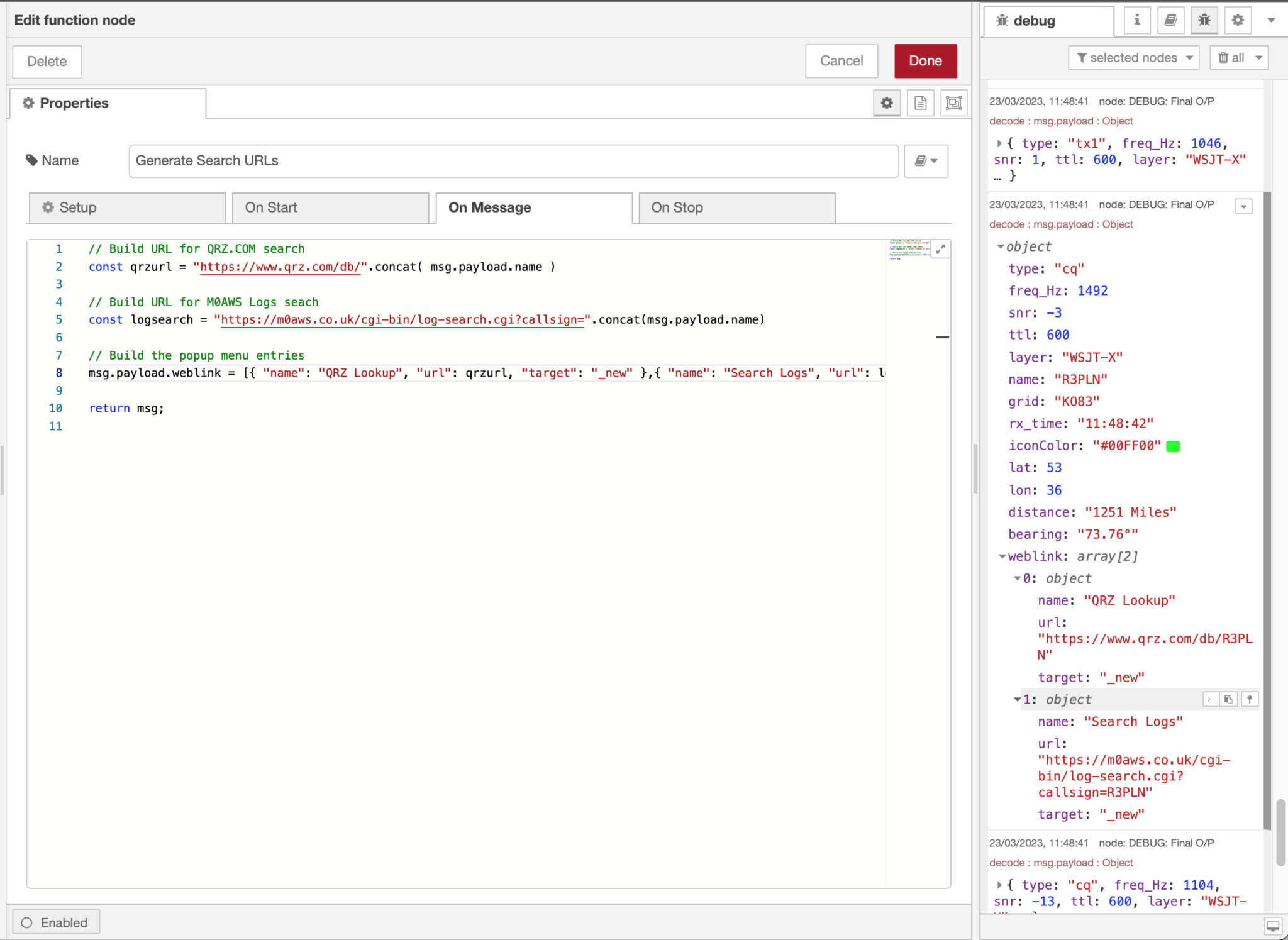
Generate Search URLs – Generates the URLs for QRZ and my own online log lookups
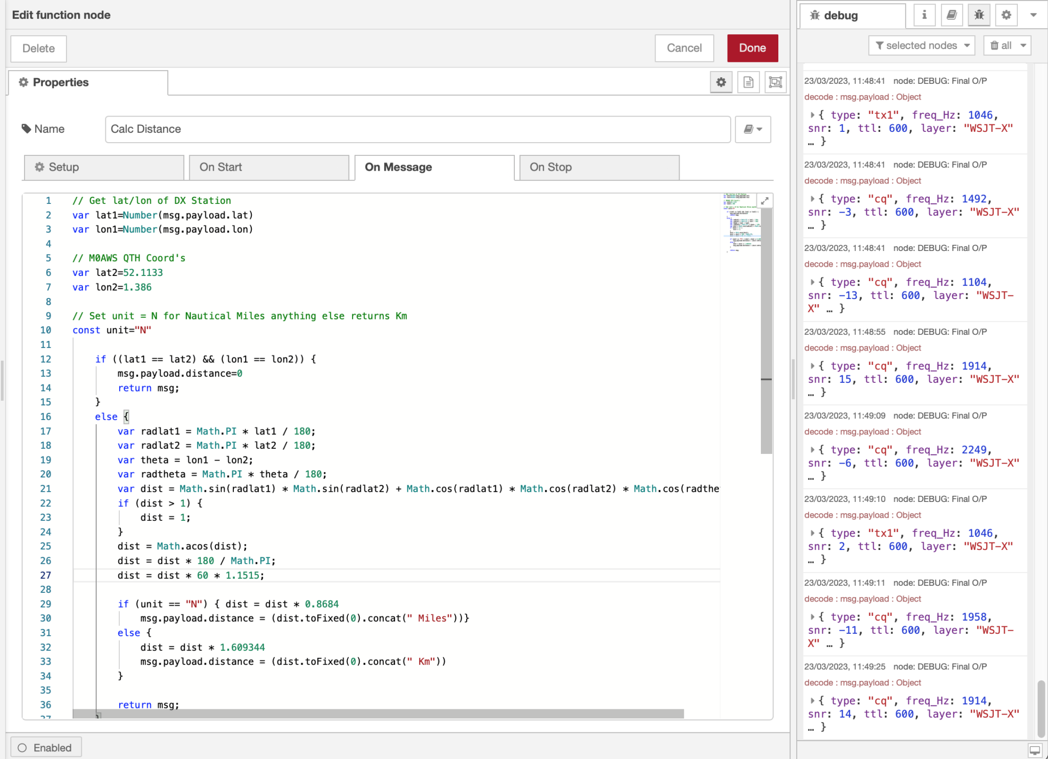
Editing the Calc Distance function with debug info in the far right panel
Once all the functions have run the resultant data set is forwarded on to the WSJT-X Stations Map node where it is plotted real time on a world map.
To view the map point your web browser at your PC running Node Red as follows:
http://radiopc.your.domain:1880/worldmap/
Or if you haven’t got a DNS setup at home then just use the IP Address of the PC instead:
http://192.168.100.10:1880/worldmap/
Don’t forget that for all of this to work you must configure WSJT-X to send data via UDP on port 2237 otherwise the flow won’t be able to connect and listen for the decode data.
You may have noticed that there are 3 other nodes that I haven’t mentioned yet. The two green greyed out nodes are Debug nodes that can be enabled when required to help see what is going on in the flow. These debug nodes will display data in the debug panel on the right of the flow editor screen when they are enabled, they are extremely useful for debugging!
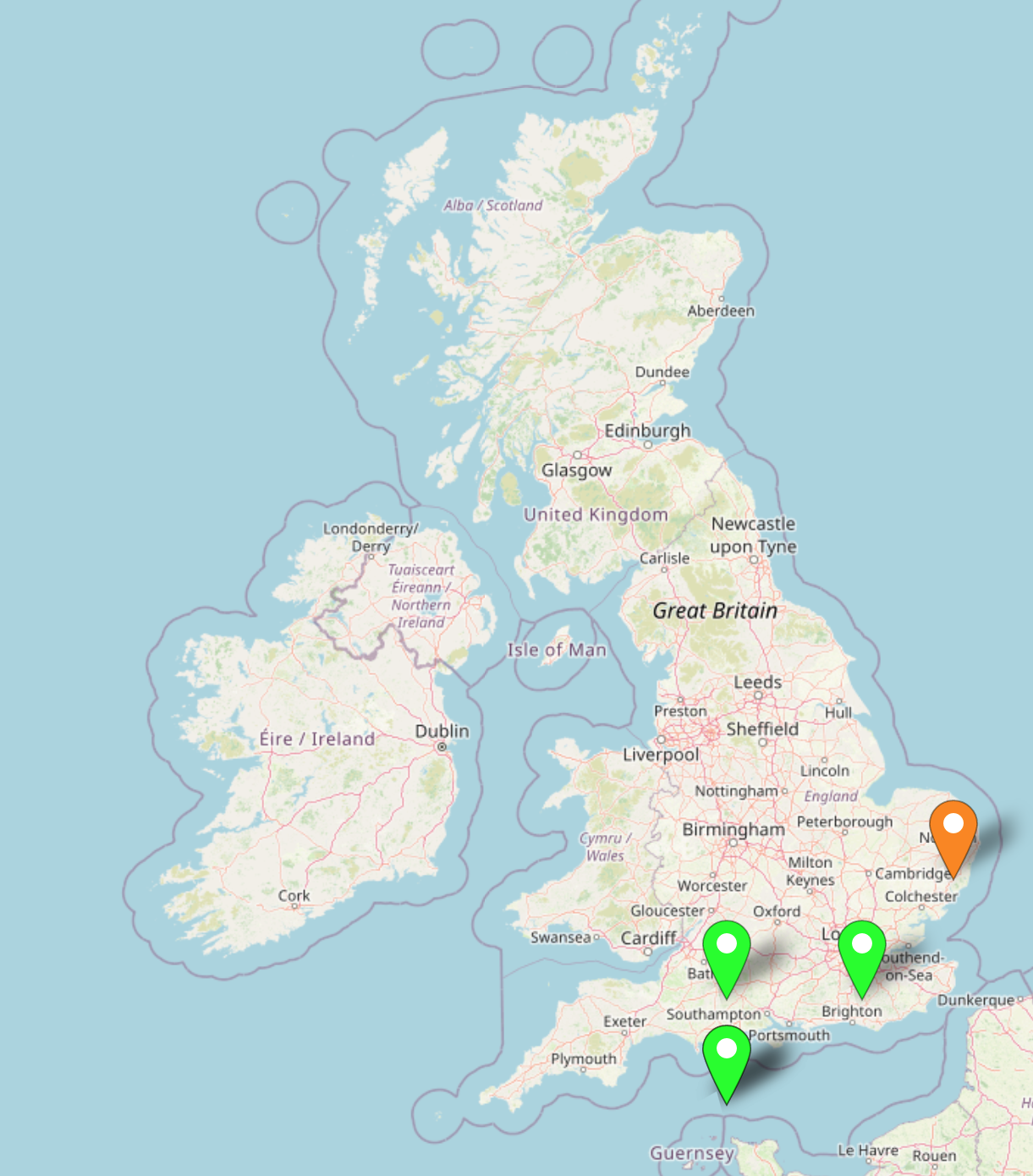
The third is the blue My QTH node, this contains data pertaining to my QTH that is plotted on the map using an orange icon. You can easily edit this node to point to your QTH instead.
WSJT-X Node Red map showing orange icon denoting my QTH
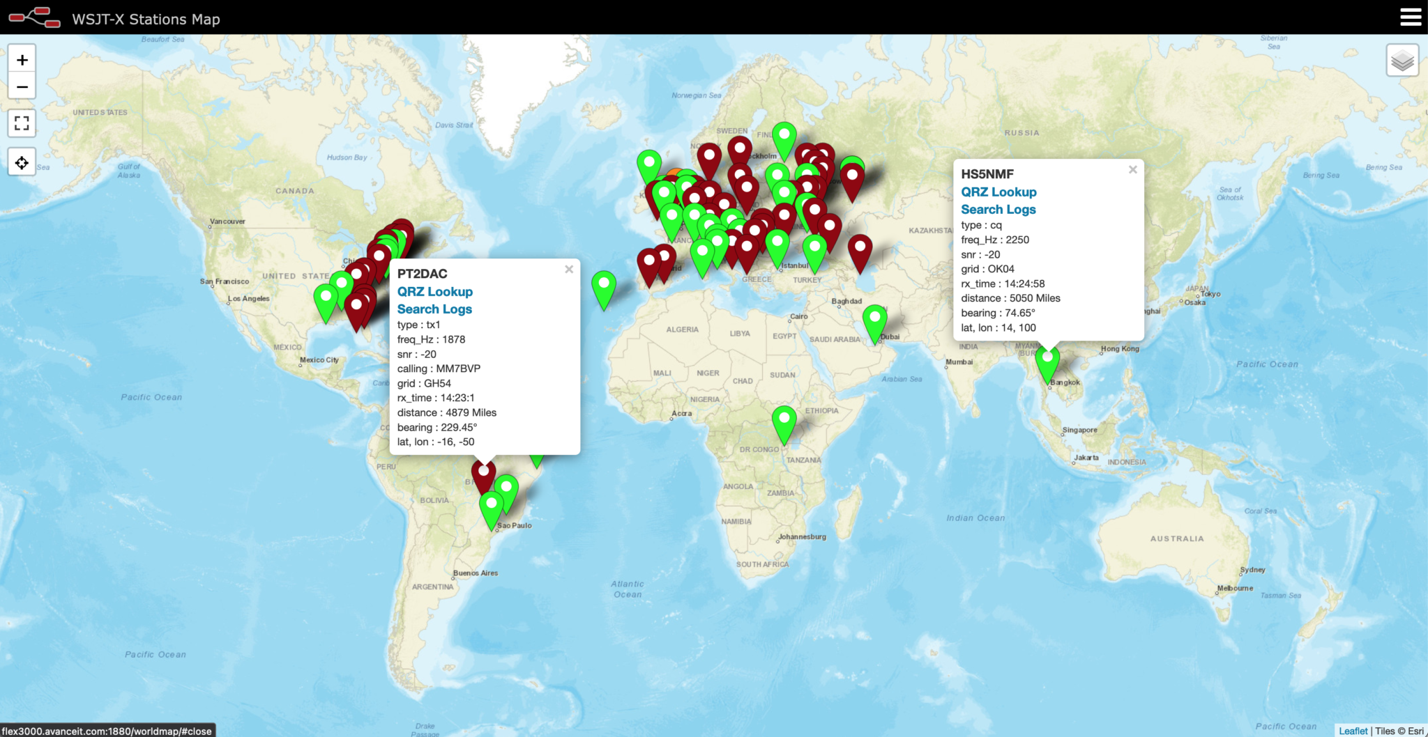
Once the flow is deployed you’ll be surprised how quickly the data starts to be plotted on the map. Stations calling “CQ” are shown by Green icons and stations that are in a QSO with another station are denoted by the Red icons.
Each icon is clickable and will present all the information collected by WSJT-X for each station viewed.
WSJT-X Node Red World Map showing FT8 stations realtime on the 12m Band
The popup also has two clickable entries, one will take you to the qrz.com page for the station being viewed and the other will search my logs to see if I have worked that station already and if so it will open a new tab showing the information.
Node Red Function Editor showing the Generate Search URLs function
You can edit the “Generate Search URLs” node so that it points to your online logs search engine so that you can view your own log data instead of mine.
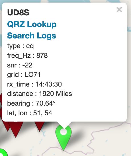
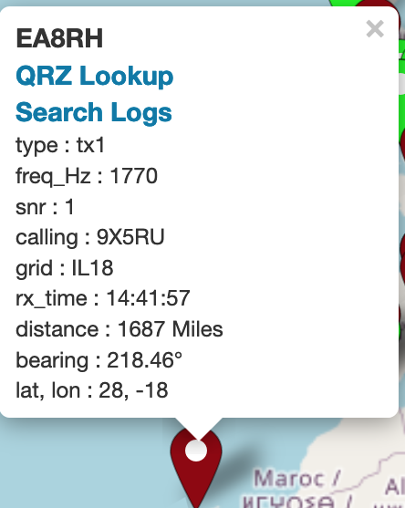
Below is a close up of the popups that are displayed when each icon on the map is clicked. The popups show the information collected from WSJT-X for each station plotted on the map.
Left – Green “CQ” Popup and Right – Red “TX1” in QSO popup
If you fancy trying this out for yourself but, don’t fancy creating all the nodes in the flow manually then I have made an export of the flow available for download. All you have to do is download the file, unzip it and then import it to Node Red and you’ll have everything built ready to play with.
I’ll probably be adding more functionality to this flow as time goes on and will post further articles about it in the future.
More soon …
We use cookies to ensure that we give you the best experience on our website. If you continue to use this site we will assume that you are happy with it.