Realtime WSJT-X decode data map

Following on from my previous article on Enhancing Digital modes with Node Red I’ve now got to a point where I have realtime decode information from the WSJT-X digital application being plotted on a Node Red world map not just for CQ calls but, for stations in conversation too.

The flow has become somewhat more complex than it was originally as more and more functionality has been added. I have deliberately split out the flow process into more nodes than are really necessary so that the flow is easier to understand. Anyone from a programming background like myself will soon realise that a lot of the nodes could actually be combined into one big node however, the overall flow process wouldn’t be so easy to understand for the Node Red newcomer and would possibly put people off from trying it out.

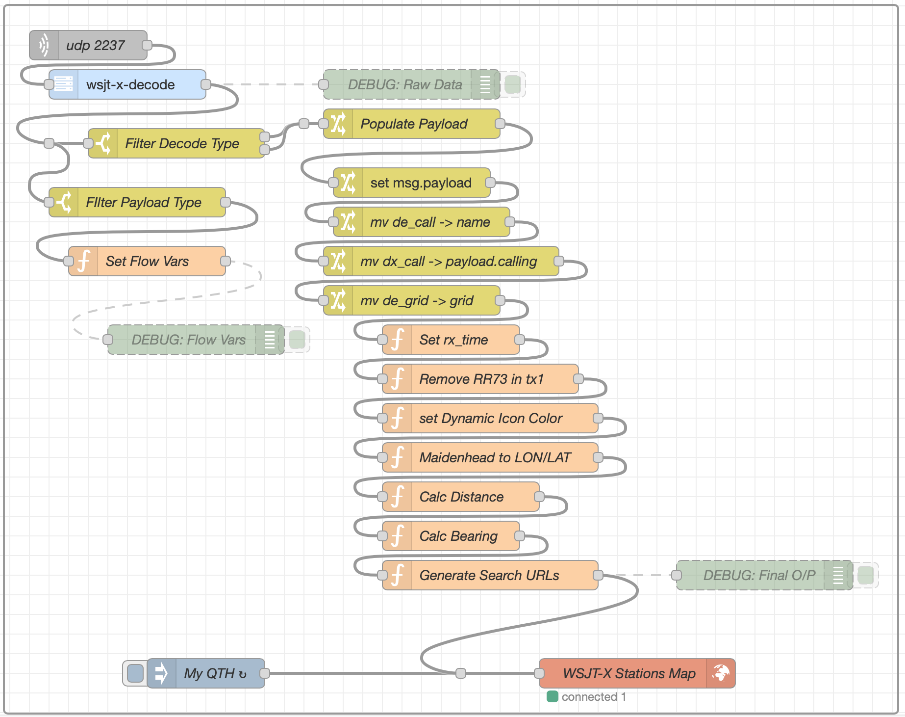
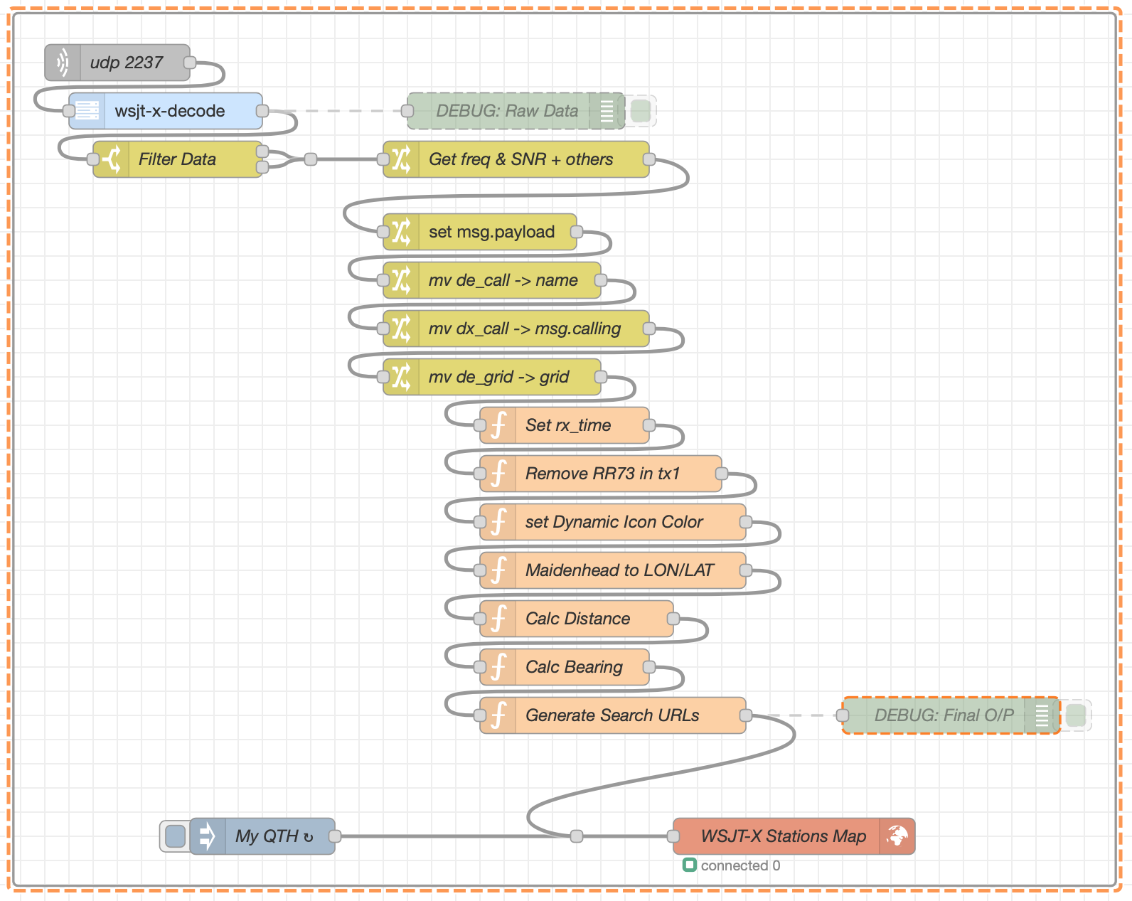
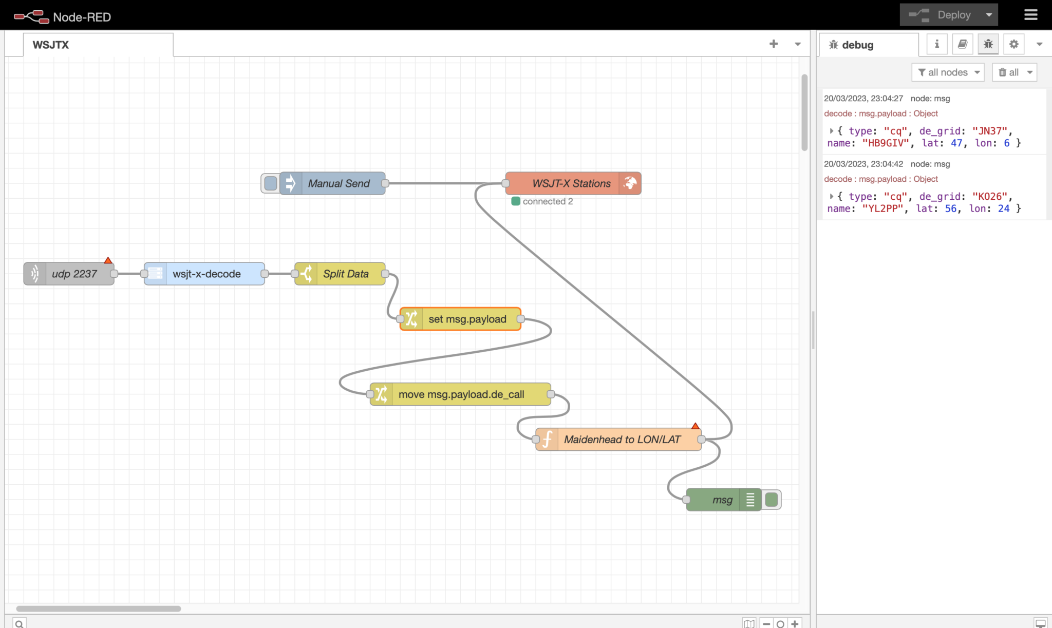
Current WSJT-X Node Red flow

Above is a screenshot of the flow as it currently stands. It’s pretty easy to understand what is happening in the flow due to the fact that the processes are broken out into small, easy to digest blocks.

From the top down we connect to WSJT-X via UDP port 2237 and listen for the data stream. As the data is received it’s passed directly into the WSJT-X-Decode node that converts the information into a Node Red compatible format. The data is then filtered with only the information required being passed onto the next node. There are two outputs from the filter node as we require two different streams of information, namely “CQ” and “TX1” data. All the rest of the data from WSJT-X is ignored as it’s not required at this time.

The “Get freq & SNR + Others” node builds a decode message payload with all the correct data, in the right format ready to be passed on along the flow. This node also sets a number of parameters required by the map node to be able to control the display of the data.

The next node along is “Set msg.payload”, this brings together all the necessary data into a single message payload that is then worked on by all the nodes further along the flow.

The next 3 nodes perform the simple task of moving some of the data into the objects defined by the world map node, if the data isn’t moved into these specific objects the map will not plot anything.

Now we get onto the slightly more difficult bit that might put off those who aren’t from a programming background. The next 7 nodes are all javascript functions which I have created to perform tasks that cannot be done via the standard Node Red pallet.

At this point it’s worth noting that I’m not a javascript programmer, I’ve used Python, Rust, Go, C and many other languages during my 40 plus year career but, javascript has never been one of them. I’m sure any seasoned javascript programmer will most likely raise an eyebrow at my attempt at javascript programming but, you need to remember that I’m doing this in my retirement and my enthusiasm for learning yet another programming language has wained somewhat!

So, getting back to the flow, each javascript function does just one task each of which is as follows:

  • Set rx_time – Sets the time the data was received/processed
  • Remove RR73 in tx1 – Remove decodes where RR73 is in TX1 instead of a valid callsign
  • Set Dynamic Icon Colour – Sets the icon colour depending on what type of call is decoded
  • Maidenhead to LON/LAT – Converts Maidenhead locator codes into LAT/LON Coordinates
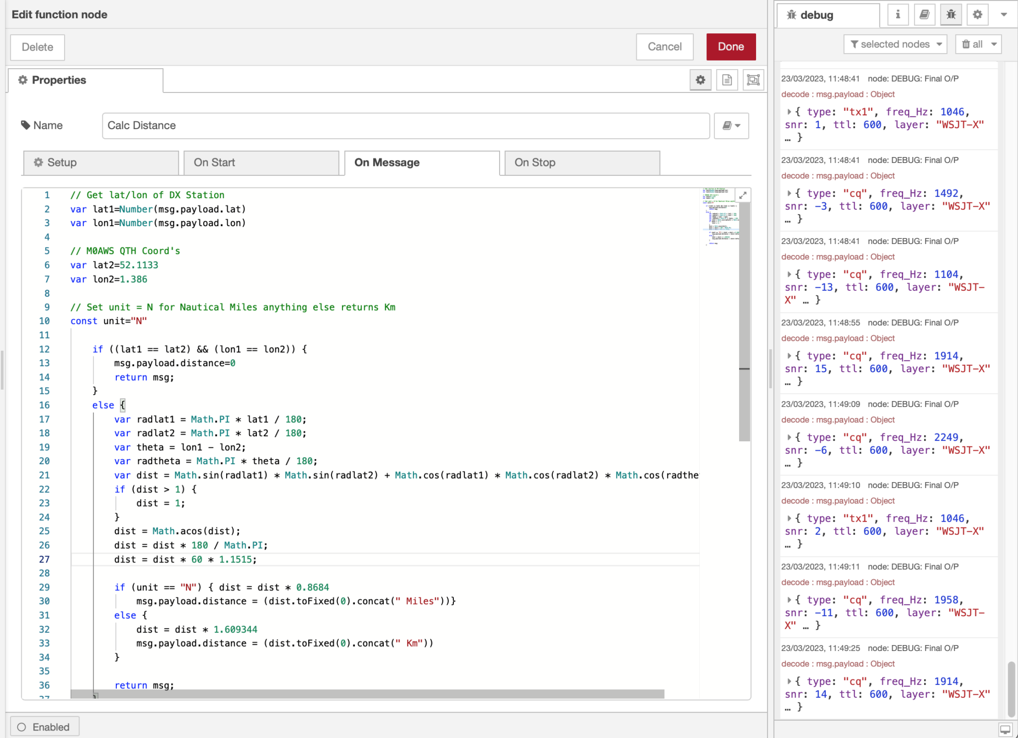
  • Calc Distance – Calculates the distance between “My QTH” and the DX station
  • Calc Bearing – Calculates the bearing/beam heading to the DX Station from “My QTH”
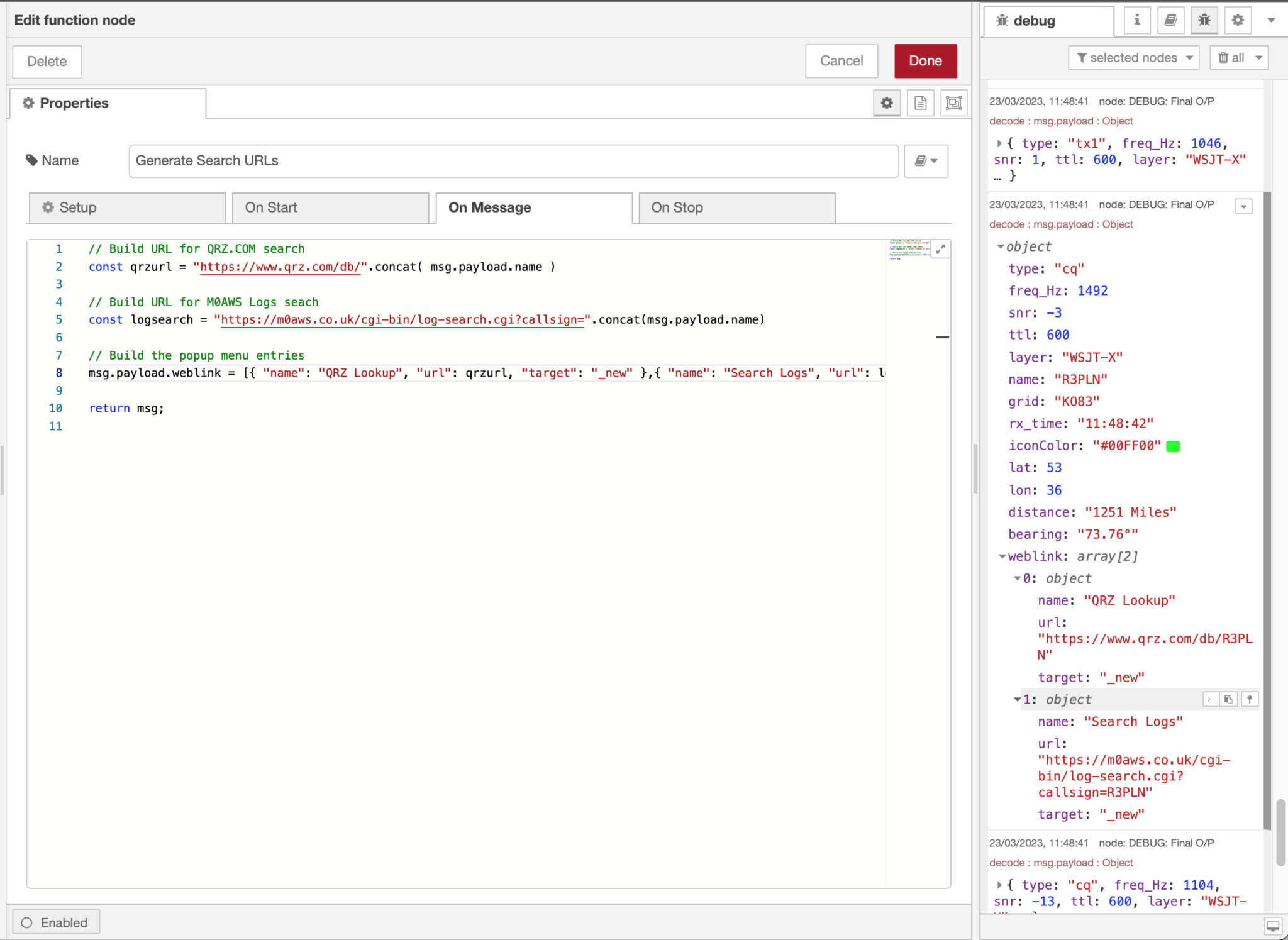
  • Generate Search URLs – Generates the URLs for QRZ and my own online log lookups
Editing the Calc Distance function with debug info in the far right panel

Once all the functions have run the resultant data set is forwarded on to the WSJT-X Stations Map node where it is plotted real time on a world map.

To view the map point your web browser at your PC running Node Red as follows:

http://radiopc.your.domain:1880/worldmap/

Or if you haven’t got a DNS setup at home then just use the IP Address of the PC instead:

http://192.168.100.10:1880/worldmap/

Don’t forget that for all of this to work you must configure WSJT-X to send data via UDP on port 2237 otherwise the flow won’t be able to connect and listen for the decode data.

You may have noticed that there are 3 other nodes that I haven’t mentioned yet. The two green greyed out nodes are Debug nodes that can be enabled when required to help see what is going on in the flow. These debug nodes will display data in the debug panel on the right of the flow editor screen when they are enabled, they are extremely useful for debugging!

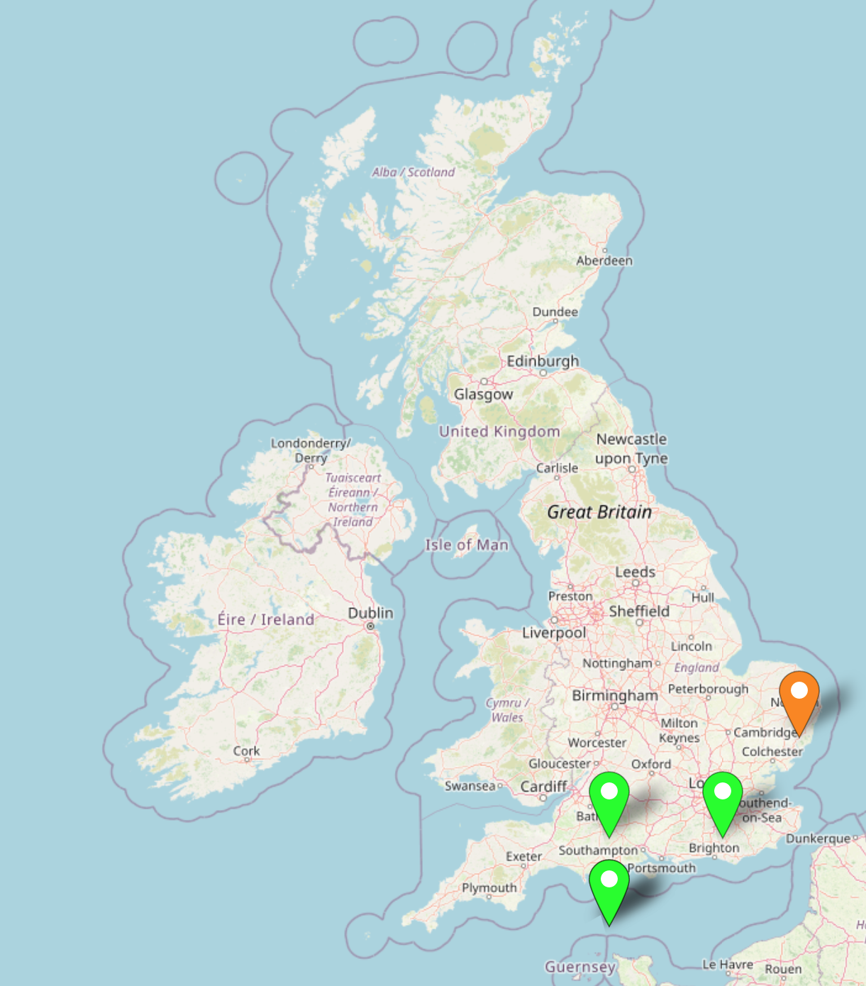
The third is the blue My QTH node, this contains data pertaining to my QTH that is plotted on the map using an orange icon. You can easily edit this node to point to your QTH instead.

WSJT-X Node Red map showing orange icon denoting my QTH

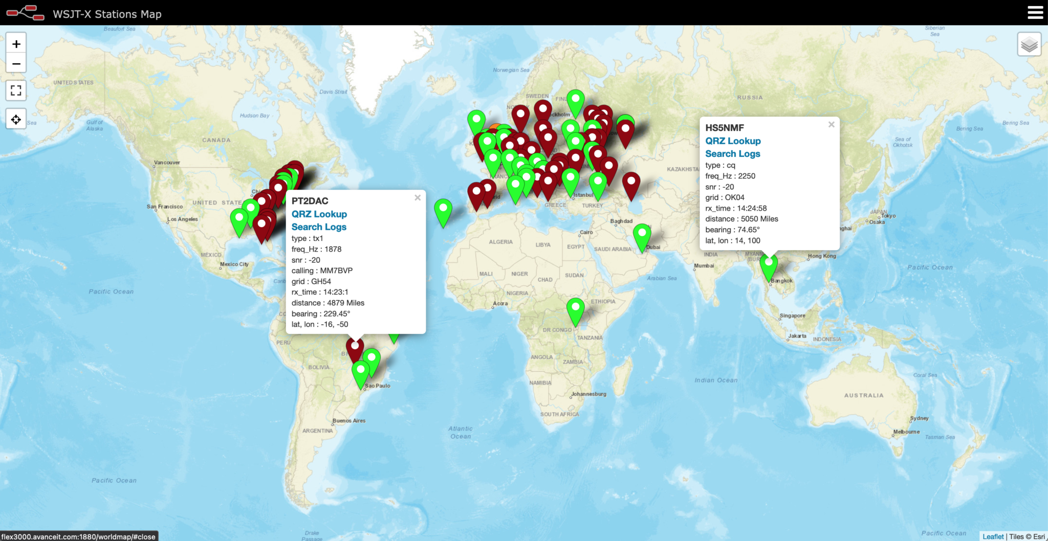
Once the flow is deployed you’ll be surprised how quickly the data starts to be plotted on the map. Stations calling “CQ” are shown by Green icons and stations that are in a QSO with another station are denoted by the Red icons.

Each icon is clickable and will present all the information collected by WSJT-X for each station viewed.

WSJT-X Node Red World Map showing FT8 stations realtime on the 12m Band

The popup also has two clickable entries, one will take you to the qrz.com page for the station being viewed and the other will search my logs to see if I have worked that station already and if so it will open a new tab showing the information.

Node Red Function Editor showing the Generate Search URLs function

You can edit the “Generate Search URLs” node so that it points to your online logs search engine so that you can view your own log data instead of mine.

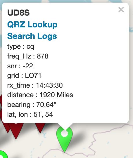
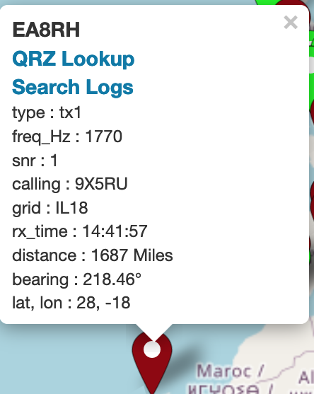
Below is a close up of the popups that are displayed when each icon on the map is clicked. The popups show the information collected from WSJT-X for each station plotted on the map.

Left – Green “CQ” Popup and Right – Red “TX1” in QSO popup

If you fancy trying this out for yourself but, don’t fancy creating all the nodes in the flow manually then I have made an export of the flow available for download. All you have to do is download the file, unzip it and then import it to Node Red and you’ll have everything built ready to play with.


I’ll probably be adding more functionality to this flow as time goes on and will post further articles about it in the future.

More soon …

Enhancing Digital modes with Node Red

For a couple of weeks now I’ve been playing with Node Red to add functionality to my digital mode applications.

To get to know how it all works I initially used Node Red to create a series of dash boards for my servers and virtual machines to show realtime information on CPU temperature, CPU load, memory usage and storage etc.

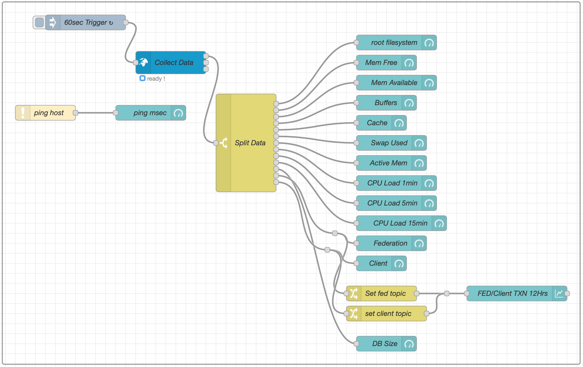
Node Red Flow to collect information from a virtual machine (VM)

This worked very well and I was soon able to generate the information I needed in a palatable format. This was a great way to get to know Node Red flow building and introduced me to using gauge and graph nodes in flows.

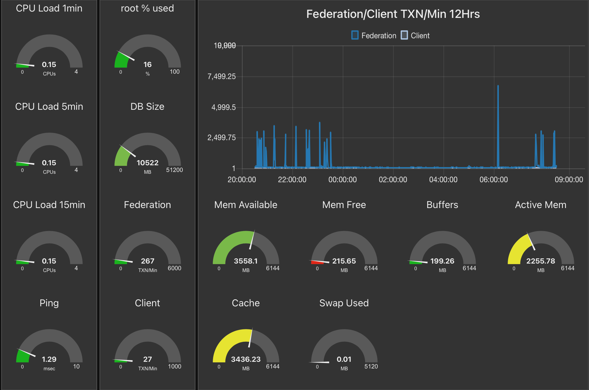
The resultant Node Red Dashboard for one of my Virtual Machines

Once I had mastered creating dashboards for servers/virtual machines (VMs) I then started to investigate using Node Red to plot data from WSJT-X on a map.

I currently use the PSKReporter website to see stations that I hear on a map as WSJT-X sends the data to the site automatically however, this information is always 5mins or more old. For some time I’ve been wanting to see the information realtime as it is received and so I was hoping to be able to achieve this via Node Red.

Node Red has nodes available for a multitude of applications all easily installed via the Manage Palette menu in the flow editor.

I installed the WSJT-X Decode and World-Map nodes and set about building a flow to capture the data and plot it on a world map.

Building a Node Red Flow to decode WSJT-X data and plot it on a World Map

Putting the building blocks of the flow together is fairly straight forward and easily achieved using the excellent flow editor built into Node Red.

I configured WSJT-X to make the decode data available via UDP on port 2237 and then started the flow by creating a UDP node that connects to WSJT-X using the same port. The data immediately started flowing and I could see the information via a debug node.

I can’t stress enough how useful debug nodes are in Node Red. You can add debug nodes onto any output on any other node to capture the data as it flows. This gives you the ability to check what you’re getting is what you expected and also to see the format the data is in. The debug data is displayed in the debug panel on the right of the flow editor in realtime and gives you a great view of what is going on in your flow.

I decided to start with capturing the data for stations calling CQ as this was easily identifiable in the JSON object coming out from WSJT-X.

Passing the output from the WSJT-X-Decode node into a switch node I added a rule that filtered out data containing “type: “cq” and passed it onto the next switch node that created a payload consisting of the station callsign, maidenhead grid square and type so that it could be passed onto the next node for processing.

The next node in the flow is a function, this is where it gets a bit tricky. To be able to plot data on the map we need the Lat/Lon coordinates of the station making the CQ call. Since WSJT-X uses maidenhead locator data I needed to convert this to Lat/Lon coordinates before passing the data to the map node to be plotted.

Since Node Red is written in Java all the functions have to be written in javascript. The problem here is that I am not a javascript programmer and so this meant I’d need to learn yet another programming language. Unfortunately Node Red doesn’t allow functions to be written in C, Rust, Go or Python, all languages that I know well and after retiring from over 40 years in the UNIX/Linux/IT world my enthusiasm for learning yet another programming language has wained somewhat.

Being so close to having a working solution I pressed on and after much head scratching I finally put together some javascript that converts the maidenhead locator information in to good old fashioned Lat/Lon coordinates. I’m sure a seasoned Javascript developer wouldn’t be impressed with my code but, it works and does what I need and so I’m happy with it for the time being.

WSJT-X FT8 stations calling CQ on the 60m Band plotted on a Node Red World Map

Once I had the location information converted it was just a matter of passing the data to the world map node in the correct format for it to be plotted realtime.

As you can see on the screenshot of the map above, it worked extremely well with stations popping up as they were decoded by WSJT-X.

I now need to refine the data sent to the map so that it shows the frequency the station is calling on, the time they made the CQ call and the mode (FT8/FT4 etc) being used.. I would also like to add the distance from my QTH to the station calling CQ to round the information off however, this will mean writing another javascript function which, I’m not sure I want to dive into just yet.

I also need to add into the mix stations that aren’t calling CQ but, who’s callsign and grid square are passed on from WSJT-X. This will mean I will then be able to add to the map those stations that are actively working other stations and maybe I might even be able to show a line between the two stations that are in QSO.

This has been a fun but, steep learning curve however, it will certainly add some great functionality into my radio room and enhance my radio HAM addiction even further.

More soon …

Funcube Dongle Pro+ / GQRX / Kubuntu

Many years ago I purchased a Funcube Dongle Pro+ (FCD) SDR. Since it’s arrival it has just been stored in my “Get round too it” drawer.

It’s been many years but, today is the day it comes out into the light and finally gets powered up.

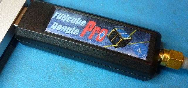
Funcube Dongle Pro+ USB SDR

I’m hoping to be able to use the FCD as the receiver in my QO-100 satellite ground station setup.

The output from the 10Ghz dish mounted LNB is around 739Mhz, well within the FCD receiver range of 150khz to 2Ghz. This will save me from having to transvert from 739Mhz to 430Mhz (70cm band) on the receive path.

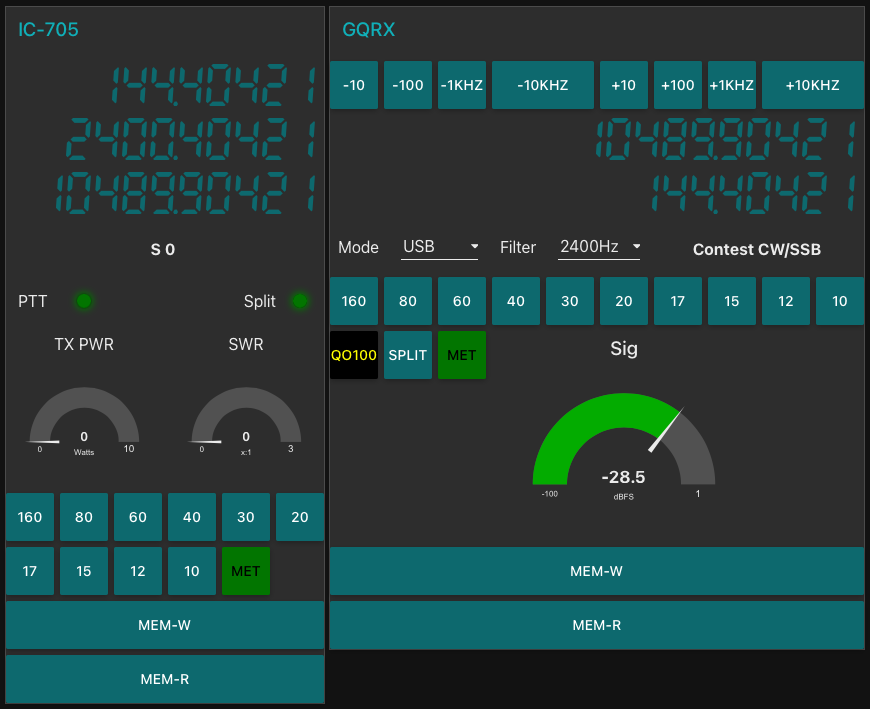
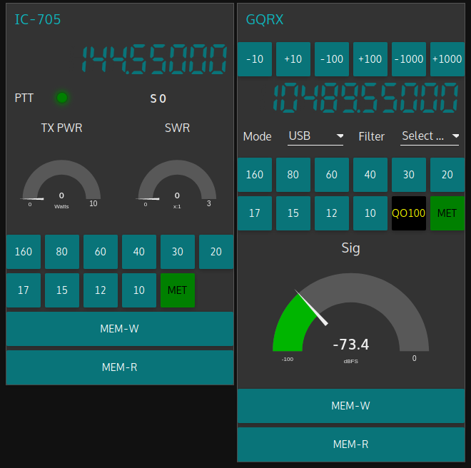
This will also give me full duplex operation as I will use my Icom IC-705 on the 2m band (144-146Mhz) to drive the 2.4Ghz transverter for the satellite uplink whilst listening to my own signal via the 10Ghz downlink fed into the FCD.

Before I can even start to build the QO-100 satellite ground station I need to get to grips with the FCD, get the software installed, configured, resolve audio routing via virtual audio cables and get it decoding FT8/JS8/WSPR etc.

Talking to G0DUB in the General Amateur Radio Chat room on Matrix he recommended trying the GQRX software to drive the FCD. GQRX is open source which fits perfectly as I want to control the FCD from my Kubuntu PC.

Checking the Ubuntu repo’s I found that GQRX v2.12 is available for installation.

sudo apt install gqrx-sdr

Once installed I fired up GQRX and set about configuring it. Initially it appeared to have automatically detected and configured the FCD however, when I started the FCD the software ran for 5 seconds and then just hung.

Diving into the configuration settings I found that the FCD actually appears twice in the list of available devices and all I had to do was select the other one in the list and start the software again and all was well.

I connected my 20m Band EFHW Vertical antenna and trawled up and down the band. The receiver performed well even with fairly strong signals so, I spent some time listening to a few of the stations coming in from the USA.

Next I wanted to sort out the configuration for digital modes. I already have a couple of virtual audio cables in the form of loopback audio devices configured on my Kubuntu PC as this is how I connect the audio between WFView for the IC-705 and WSJT-X/JS8CALL.

Sadly, GQRX doesn’t recognise the loopback audio devices that already exist and so I had to do a little further research to get to the bottom of the issue.

Digging deeper I discovered that GQRX requires loopback audio devices created using Pulse Audio and not the kind I had already created at the O/S level. A quick read of the pactl man page and some further searching online I found all the info I needed to create the correct kind of loopback audio devices.

Two commands are required to create the pulse audio server audio loopback devices:

pactl load-module module-null-sink sink_name=gq2jt sink_properties=device.description="gq2jt"

pactl load-module module-loopback latency_msec=1

Once I’d created the loopback audio devices I was able to select the gq2jt devices in both GQRX and WSJT-X/JS8CALL so that the audio was routed correctly.

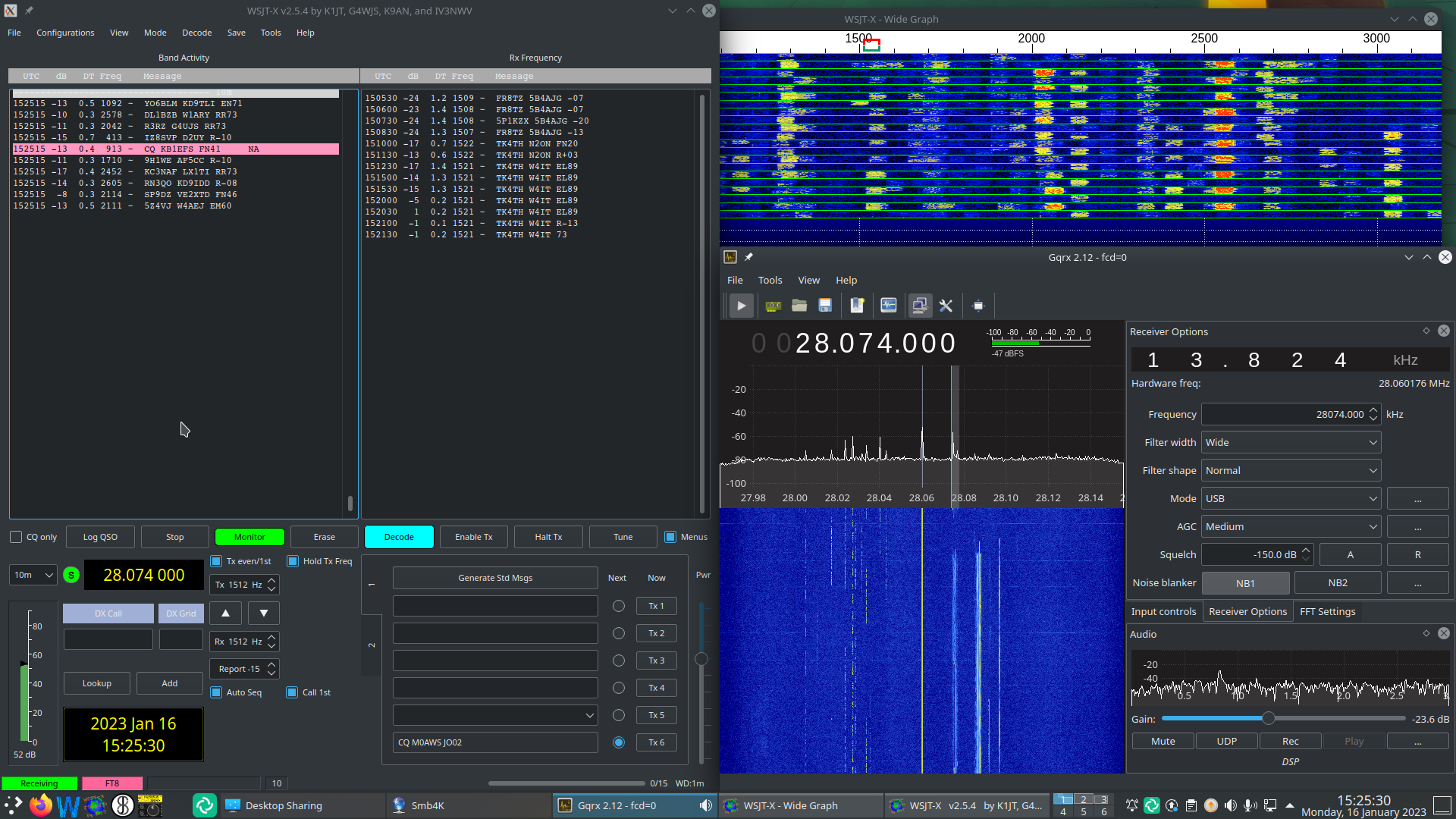
GQRX SDR and WSJT-X working with the Funcube Dongle Pro+

The overall solution works well and doesn’t put much load on the CPU of my Kubuntu PC, leaving plenty of horse power for me to do other things at the same time.

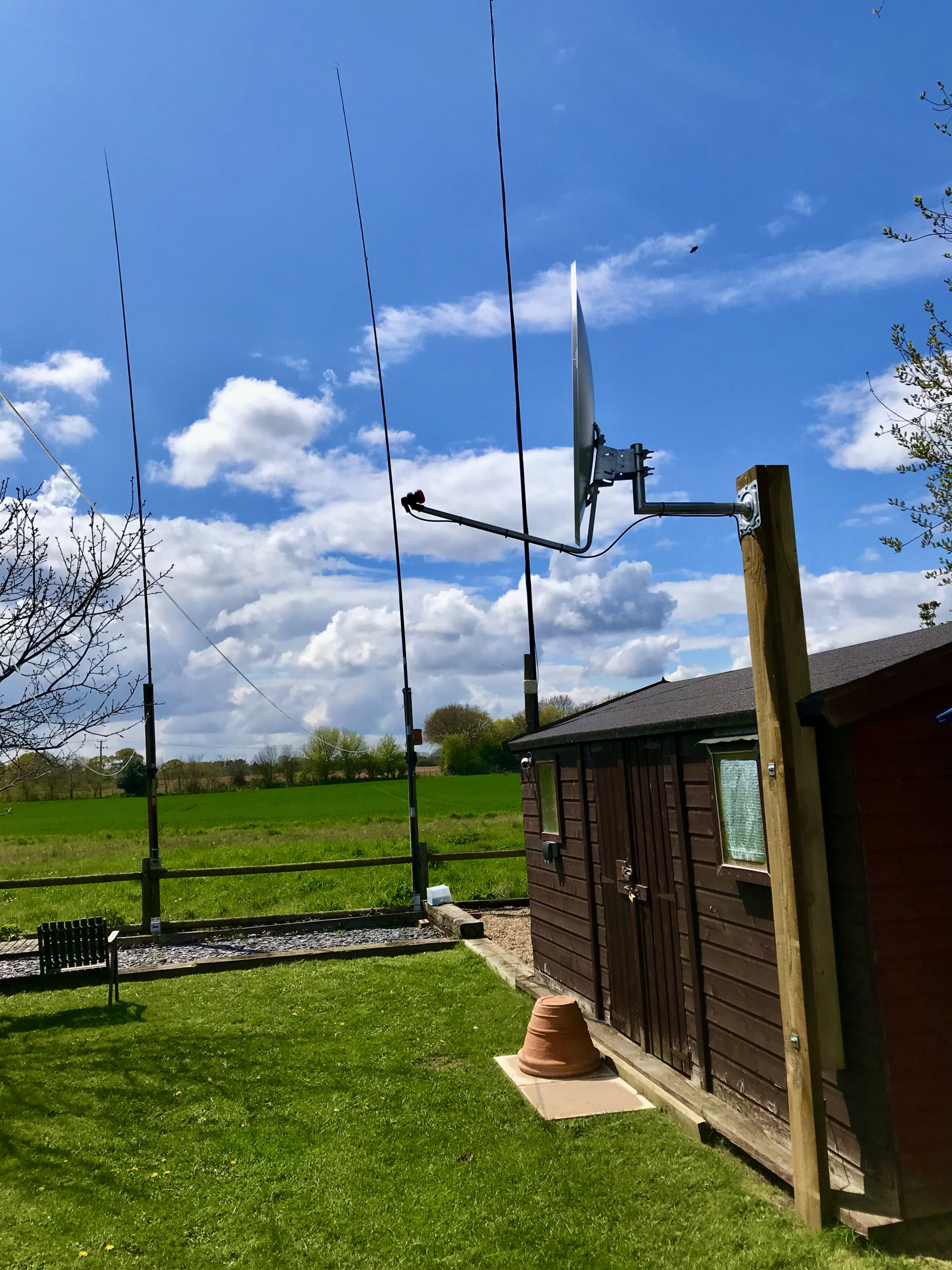
So I now have the Funcube Dongle Pro+ working perfectly on my Kubuntu PC, all I need now is a 1.2m dish, a 10Ghz LNB and some high quality coax cable.

UPDATE: I decided to leave the FCD connected to the 20m Band EFHW Vertical overnight and monitor FT8 on the 40m band. The EFHW antenna isn’t anywhere near resonant on the 40m band and so I thought it would be interesting to see how well the FCD performed on a completely non-resonant antenna.

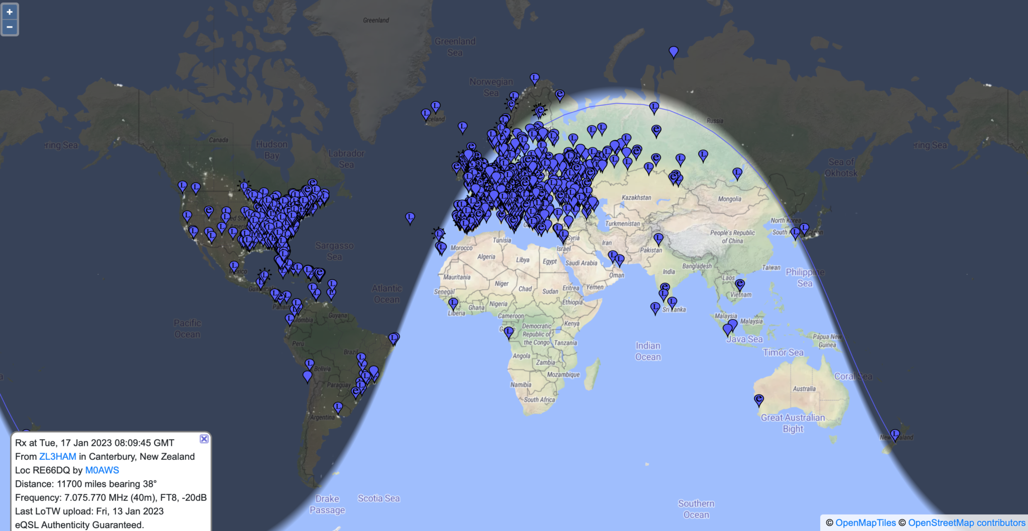
To my surprise it did exceptionally well, stations from all over the world were heard with ease, the FCD really is an excellent little SDR receiver.

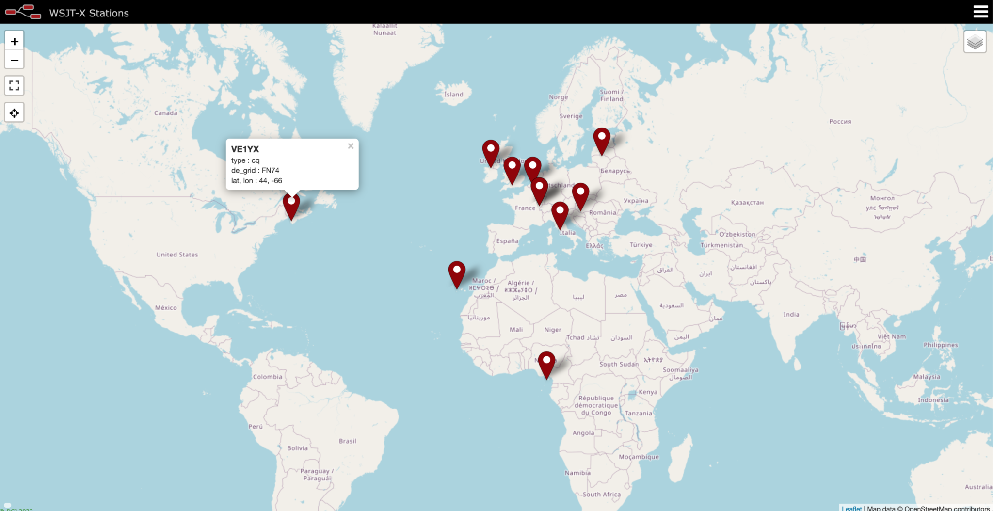
Map showing stations heard on 40m Band FT8 over night 16/17 Jan 2023

If you’re looking for a relatively cheap but, effective receiver for FT8/WSPR monitoring then I can highly recommend the FCD. If paired with a RaspberryPi then it would be a really cheap to purchase/operate solution for any HAM operator or short wave listener (SWL).

More soon …

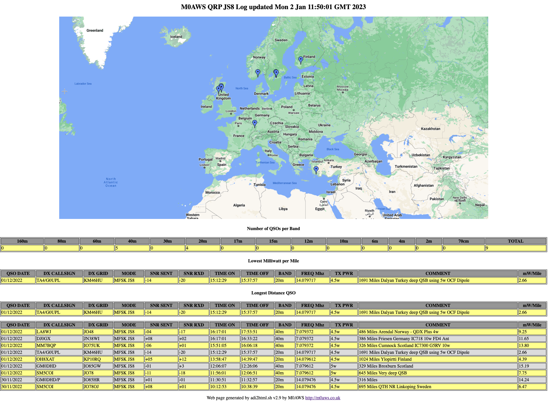
JS8 Logs now online

I’ve now added my JS8/JS8CALL logs to the website for both QRO (25w Max) and QRP (<10w) QSOs.

The JS8 logs are available from the Logs menu above.

I’ve updated the adi2html program to now be capable of processing the JS8CALL log file and will be releasing it into the public domain soon.

M0AWS QRP JS8 Online Log

More soon …

Getting chatty with JS8CALL

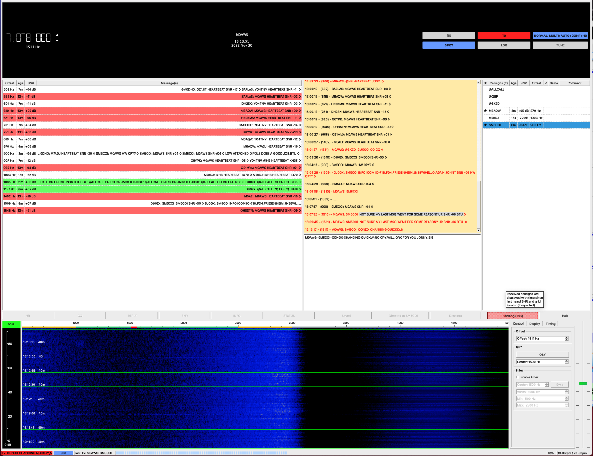
JS8CALL running on my MacBook Pro

I’ve been chasing the DX on the HF bands using FT8 for a while now and I have to say it’s been very successful however, it does get rather boring after a while just exchanging SNR reports and nothing else. I noticed that my time spent in the shack was getting less and less, not a good sign after all the work I’d put into building the new radio shack.

Since there’s not a lot of CW on the bands these days (everyone is on FT8) I thought I’d give JS8CALL a go.

Initially I started with trying to get JS8CALL working on my Kubuntu PC to my Icom IC-705 wirelessly. This turned out not to be as straight forward as I’d hoped but, I persevered.

I found that to communicate with the IC-705 via WFview wirelessly I needed to use FLRig as a go between. I installed FLRig from the Ubuntu repo’s only to find it’s an old version that doesn’t have support for the IC-705. Downloading the IC-705.xml file didn’t help either so I uninstalled it and headed to the source forge website to grab the source code for the latest version of FLRig.

Once I had the right development libraries installed compiling the code was easy enough and I soon had FLRig talking to the IC-705 via WFview wirelessly from my Kubuntu PC.

My first JS8 QSO was with Jonny, SM5COI in Sweden on the 20m band, using just 2.5w I had a very reliable link from my 20m band EFHW vertical antenna to his 20m band yagi antenna.

I also worked GM0DHD/P via OH8XAT using the relay capability built into JS8CALL, it works incredibly well and allows you to work the stations that you cannot hear directly, very useful!

Later in the morning Jonny, SM5COI emailed me asking for a sked on the 40m band later in the afternoon, of course I agreed and decided that I’d also get my MacBook Pro setup with JS8CALL so I could give my Yaesu FTDX10 a spin on JS8 mode.

Installing and configuring JS8CALL on my MacBook Pro was much easier and I had it fully operational in minutes.

The sked went well on 40m and it was good to get Jonny on another band.

With 3 JS8 QSOs in the log it’s great to be using a digital mode again that allows you to have a good chat with other radio HAMs around the world. I think this may become my preferred digital mode going forward.

More soon…