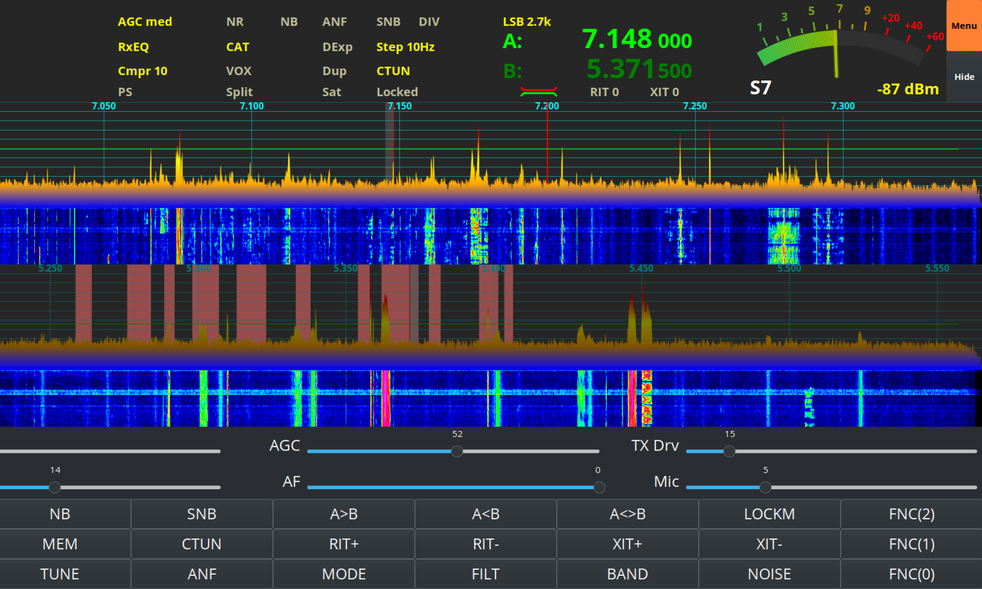
Enhancing Digital modes with Node Red

For a couple of weeks now I’ve been playing with Node Red to add functionality to my digital mode applications.

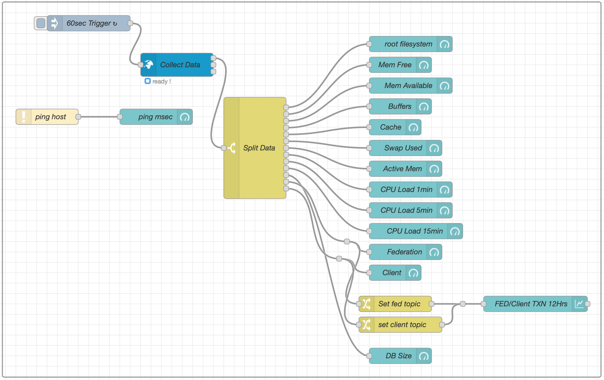
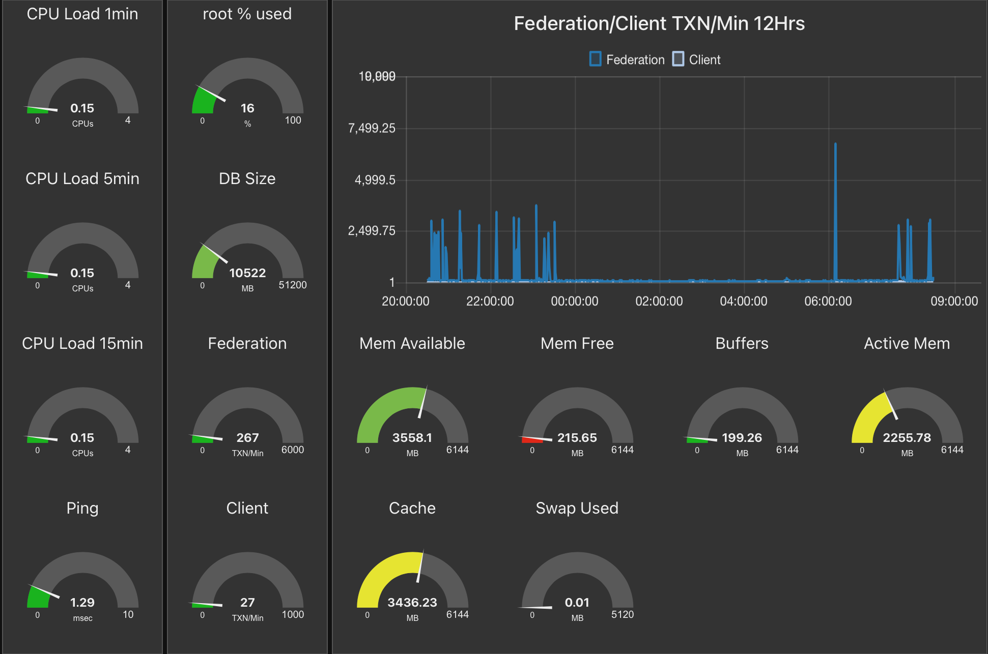
To get to know how it all works I initially used Node Red to create a series of dash boards for my servers and virtual machines to show realtime information on CPU temperature, CPU load, memory usage and storage etc.

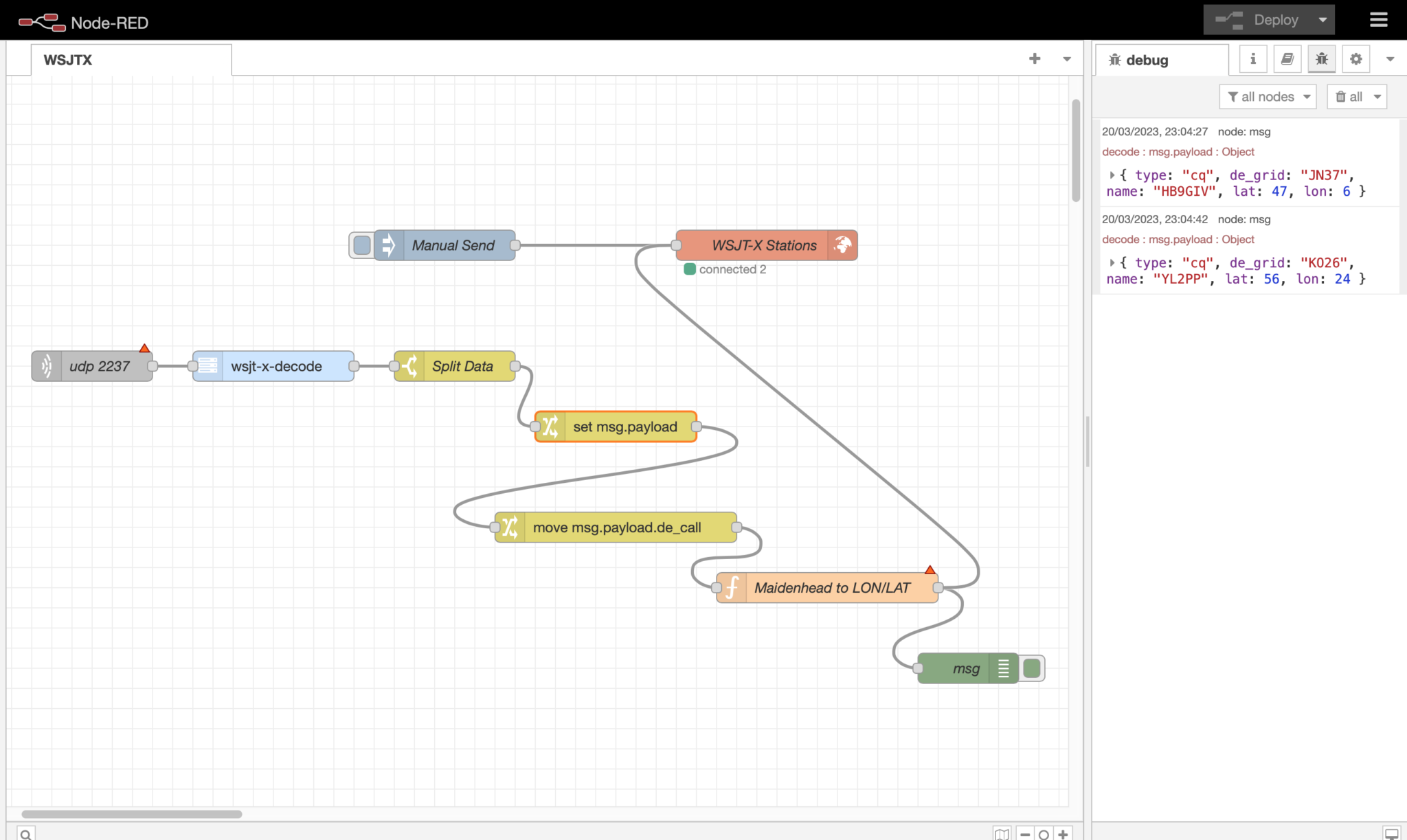
Node Red Flow to collect information from a virtual machine (VM)

This worked very well and I was soon able to generate the information I needed in a palatable format. This was a great way to get to know Node Red flow building and introduced me to using gauge and graph nodes in flows.

The resultant Node Red Dashboard for one of my Virtual Machines

Once I had mastered creating dashboards for servers/virtual machines (VMs) I then started to investigate using Node Red to plot data from WSJT-X on a map.

I currently use the PSKReporter website to see stations that I hear on a map as WSJT-X sends the data to the site automatically however, this information is always 5mins or more old. For some time I’ve been wanting to see the information realtime as it is received and so I was hoping to be able to achieve this via Node Red.

Node Red has nodes available for a multitude of applications all easily installed via the Manage Palette menu in the flow editor.

I installed the WSJT-X Decode and World-Map nodes and set about building a flow to capture the data and plot it on a world map.

Building a Node Red Flow to decode WSJT-X data and plot it on a World Map

Putting the building blocks of the flow together is fairly straight forward and easily achieved using the excellent flow editor built into Node Red.

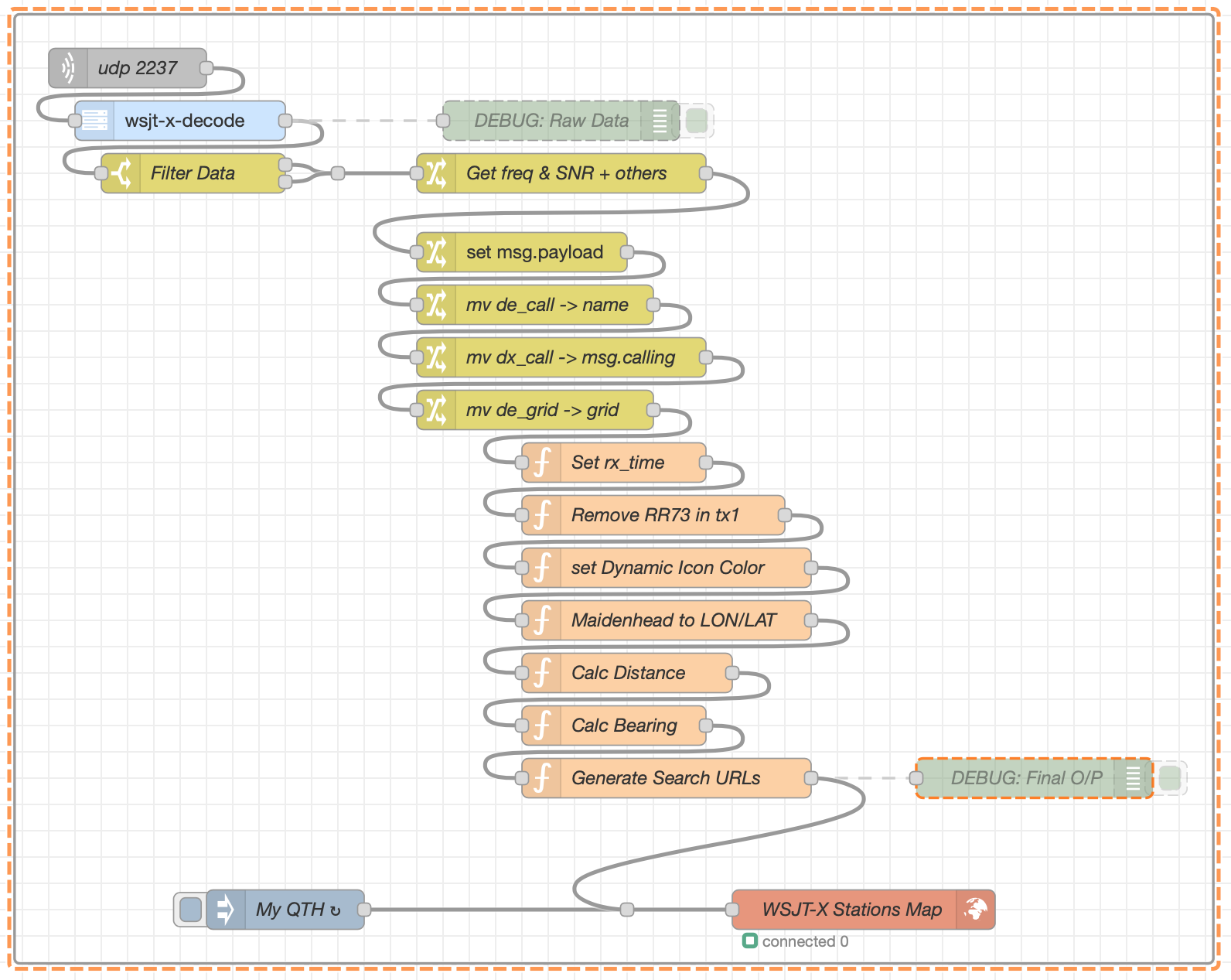
I configured WSJT-X to make the decode data available via UDP on port 2237 and then started the flow by creating a UDP node that connects to WSJT-X using the same port. The data immediately started flowing and I could see the information via a debug node.

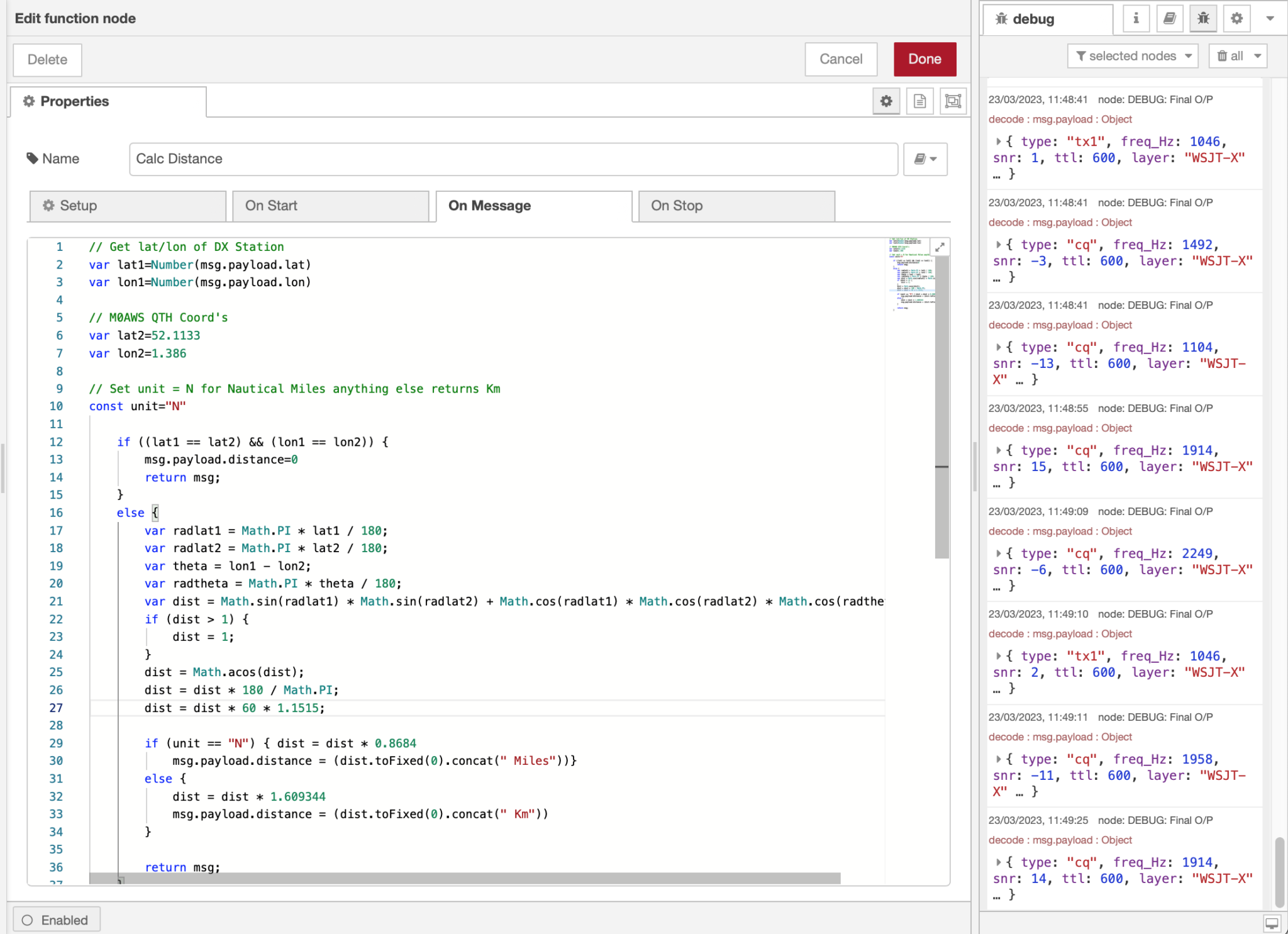
I can’t stress enough how useful debug nodes are in Node Red. You can add debug nodes onto any output on any other node to capture the data as it flows. This gives you the ability to check what you’re getting is what you expected and also to see the format the data is in. The debug data is displayed in the debug panel on the right of the flow editor in realtime and gives you a great view of what is going on in your flow.

I decided to start with capturing the data for stations calling CQ as this was easily identifiable in the JSON object coming out from WSJT-X.

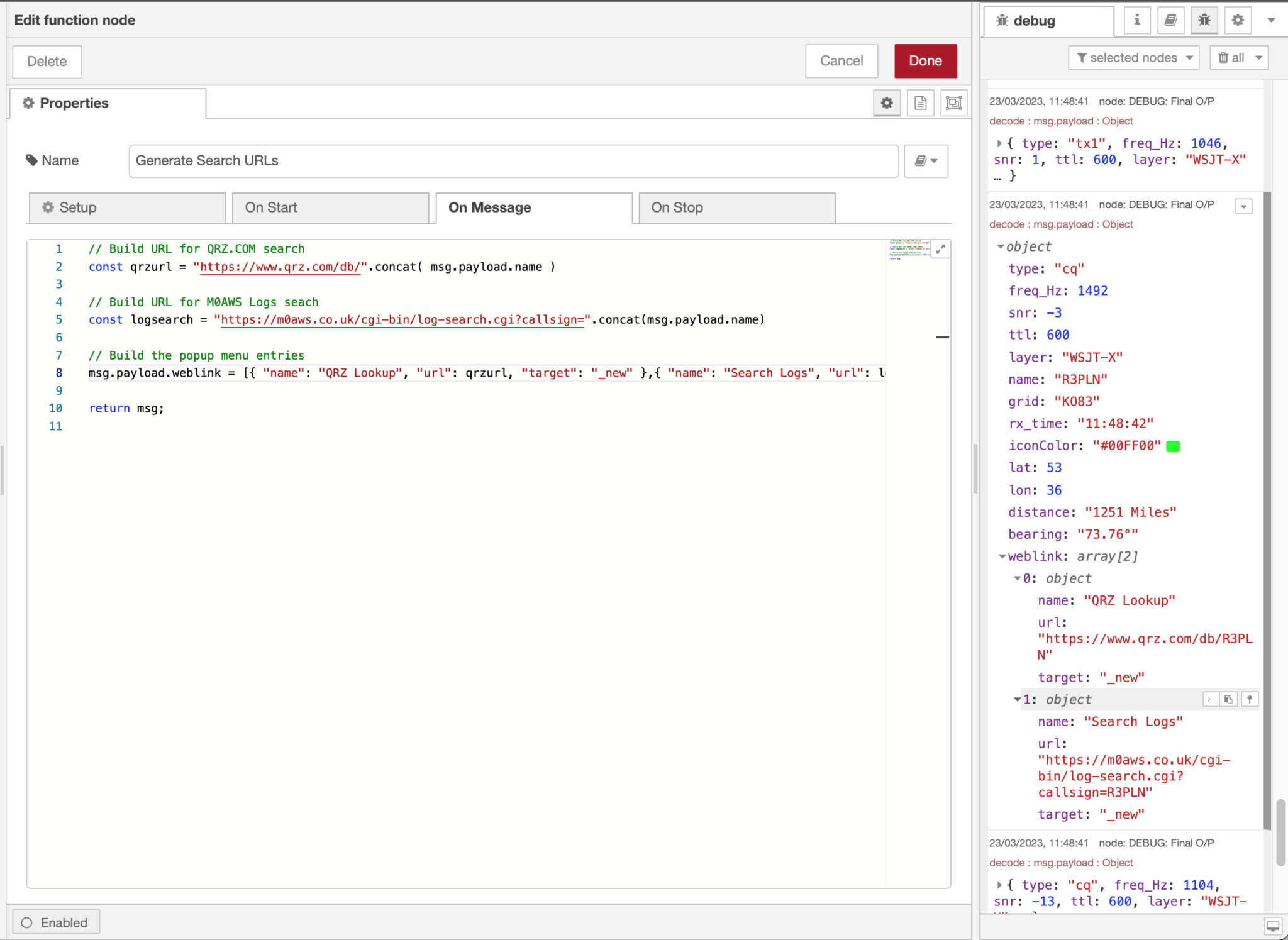
Passing the output from the WSJT-X-Decode node into a switch node I added a rule that filtered out data containing “type: “cq” and passed it onto the next switch node that created a payload consisting of the station callsign, maidenhead grid square and type so that it could be passed onto the next node for processing.

The next node in the flow is a function, this is where it gets a bit tricky. To be able to plot data on the map we need the Lat/Lon coordinates of the station making the CQ call. Since WSJT-X uses maidenhead locator data I needed to convert this to Lat/Lon coordinates before passing the data to the map node to be plotted.

Since Node Red is written in Java all the functions have to be written in javascript. The problem here is that I am not a javascript programmer and so this meant I’d need to learn yet another programming language. Unfortunately Node Red doesn’t allow functions to be written in C, Rust, Go or Python, all languages that I know well and after retiring from over 40 years in the UNIX/Linux/IT world my enthusiasm for learning yet another programming language has wained somewhat.

Being so close to having a working solution I pressed on and after much head scratching I finally put together some javascript that converts the maidenhead locator information in to good old fashioned Lat/Lon coordinates. I’m sure a seasoned Javascript developer wouldn’t be impressed with my code but, it works and does what I need and so I’m happy with it for the time being.

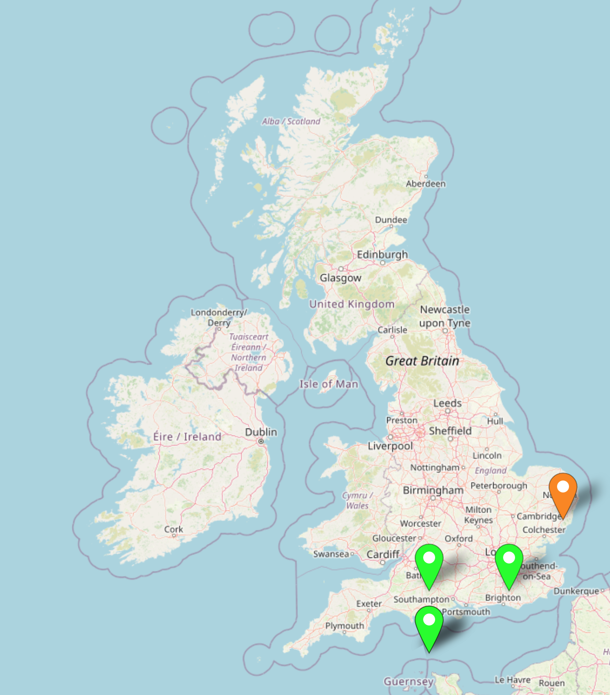
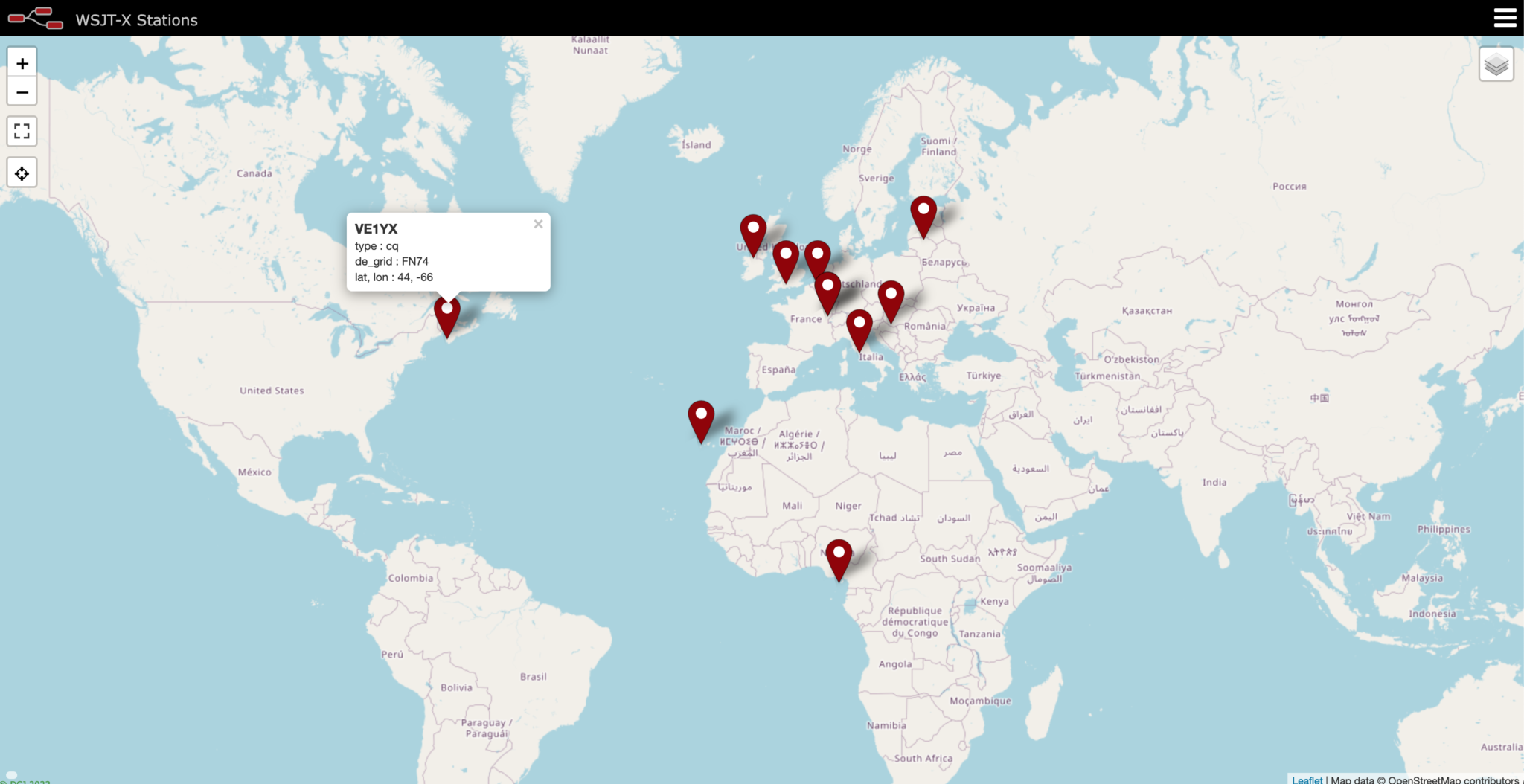
WSJT-X FT8 stations calling CQ on the 60m Band plotted on a Node Red World Map

Once I had the location information converted it was just a matter of passing the data to the world map node in the correct format for it to be plotted realtime.

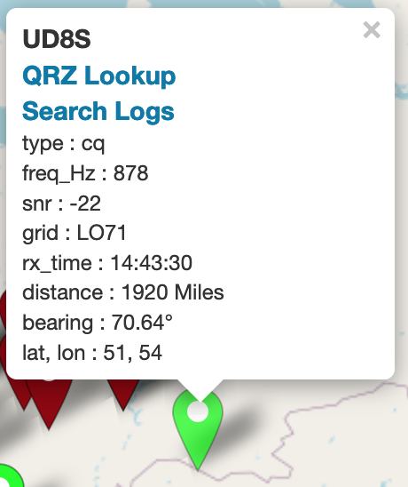
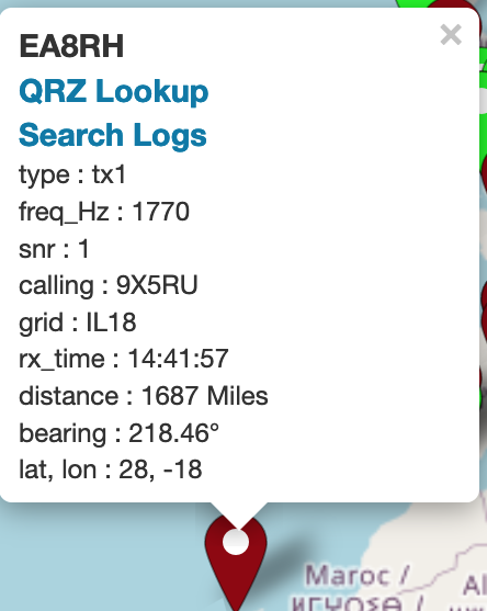
As you can see on the screenshot of the map above, it worked extremely well with stations popping up as they were decoded by WSJT-X.

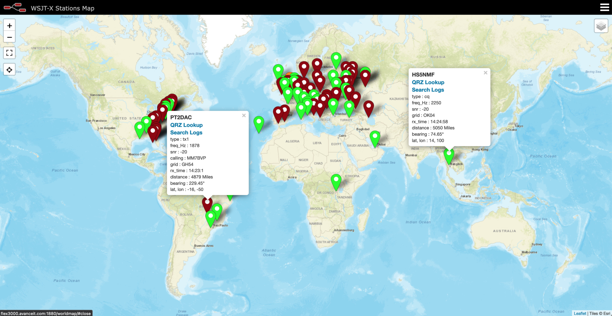
I now need to refine the data sent to the map so that it shows the frequency the station is calling on, the time they made the CQ call and the mode (FT8/FT4 etc) being used.. I would also like to add the distance from my QTH to the station calling CQ to round the information off however, this will mean writing another javascript function which, I’m not sure I want to dive into just yet.

I also need to add into the mix stations that aren’t calling CQ but, who’s callsign and grid square are passed on from WSJT-X. This will mean I will then be able to add to the map those stations that are actively working other stations and maybe I might even be able to show a line between the two stations that are in QSO.

This has been a fun but, steep learning curve however, it will certainly add some great functionality into my radio room and enhance my radio HAM addiction even further.

More soon …
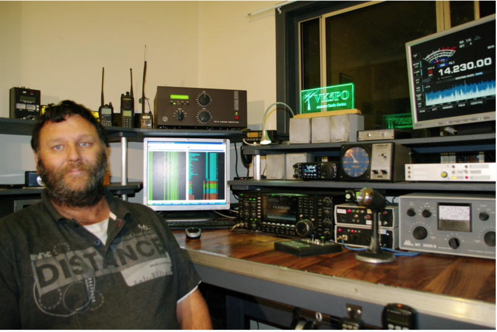
Funcube Dongle Pro+ / GQRX / Kubuntu

Many years ago I purchased a Funcube Dongle Pro+ (FCD) SDR. Since it’s arrival it has just been stored in my “Get round too it” drawer.

It’s been many years but, today is the day it comes out into the light and finally gets powered up.

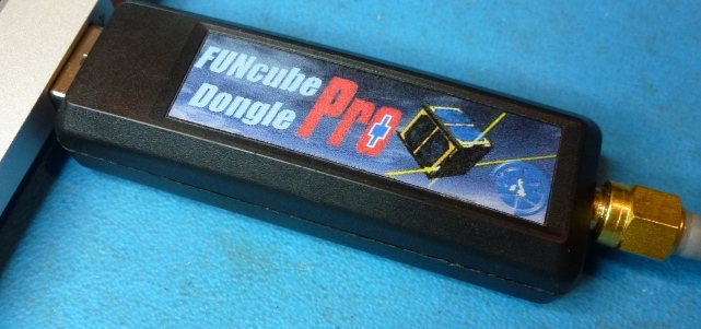
Funcube Dongle Pro+ USB SDR

I’m hoping to be able to use the FCD as the receiver in my QO-100 satellite ground station setup.

The output from the 10Ghz dish mounted LNB is around 739Mhz, well within the FCD receiver range of 150khz to 2Ghz. This will save me from having to transvert from 739Mhz to 430Mhz (70cm band) on the receive path.

This will also give me full duplex operation as I will use my Icom IC-705 on the 2m band (144-146Mhz) to drive the 2.4Ghz transverter for the satellite uplink whilst listening to my own signal via the 10Ghz downlink fed into the FCD.

Before I can even start to build the QO-100 satellite ground station I need to get to grips with the FCD, get the software installed, configured, resolve audio routing via virtual audio cables and get it decoding FT8/JS8/WSPR etc.

Talking to G0DUB in the General Amateur Radio Chat room on Matrix he recommended trying the GQRX software to drive the FCD. GQRX is open source which fits perfectly as I want to control the FCD from my Kubuntu PC.

Checking the Ubuntu repo’s I found that GQRX v2.12 is available for installation.

sudo apt install gqrx-sdr

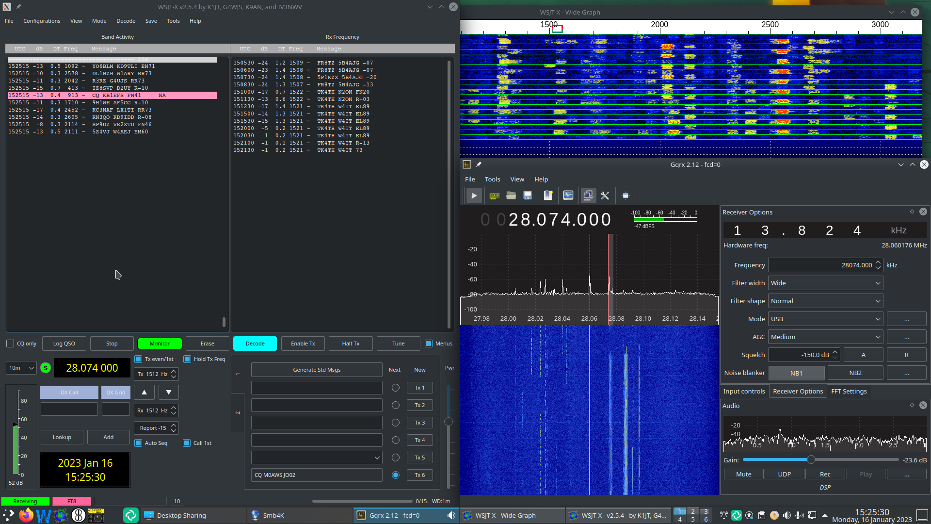
Once installed I fired up GQRX and set about configuring it. Initially it appeared to have automatically detected and configured the FCD however, when I started the FCD the software ran for 5 seconds and then just hung.

Diving into the configuration settings I found that the FCD actually appears twice in the list of available devices and all I had to do was select the other one in the list and start the software again and all was well.

I connected my 20m Band EFHW Vertical antenna and trawled up and down the band. The receiver performed well even with fairly strong signals so, I spent some time listening to a few of the stations coming in from the USA.

Next I wanted to sort out the configuration for digital modes. I already have a couple of virtual audio cables in the form of loopback audio devices configured on my Kubuntu PC as this is how I connect the audio between WFView for the IC-705 and WSJT-X/JS8CALL.

Sadly, GQRX doesn’t recognise the loopback audio devices that already exist and so I had to do a little further research to get to the bottom of the issue.

Digging deeper I discovered that GQRX requires loopback audio devices created using Pulse Audio and not the kind I had already created at the O/S level. A quick read of the pactl man page and some further searching online I found all the info I needed to create the correct kind of loopback audio devices.

Two commands are required to create the pulse audio server audio loopback devices:

pactl load-module module-null-sink sink_name=gq2jt sink_properties=device.description="gq2jt"

pactl load-module module-loopback latency_msec=1

Once I’d created the loopback audio devices I was able to select the gq2jt devices in both GQRX and WSJT-X/JS8CALL so that the audio was routed correctly.

GQRX SDR and WSJT-X working with the Funcube Dongle Pro+

The overall solution works well and doesn’t put much load on the CPU of my Kubuntu PC, leaving plenty of horse power for me to do other things at the same time.

So I now have the Funcube Dongle Pro+ working perfectly on my Kubuntu PC, all I need now is a 1.2m dish, a 10Ghz LNB and some high quality coax cable.

UPDATE: I decided to leave the FCD connected to the 20m Band EFHW Vertical overnight and monitor FT8 on the 40m band. The EFHW antenna isn’t anywhere near resonant on the 40m band and so I thought it would be interesting to see how well the FCD performed on a completely non-resonant antenna.

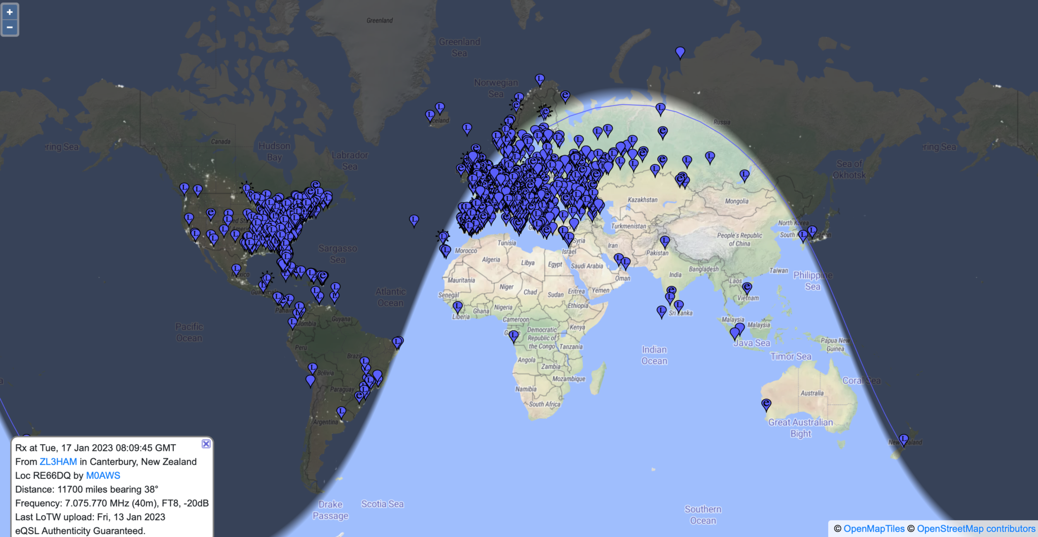
To my surprise it did exceptionally well, stations from all over the world were heard with ease, the FCD really is an excellent little SDR receiver.

Map showing stations heard on 40m Band FT8 over night 16/17 Jan 2023

If you’re looking for a relatively cheap but, effective receiver for FT8/WSPR monitoring then I can highly recommend the FCD. If paired with a RaspberryPi then it would be a really cheap to purchase/operate solution for any HAM operator or short wave listener (SWL).

More soon …

A Great start to 2023

The 2023 new year has got off to a great start here at the M0AWS radio shack with my first QSO with New Zealand since setting up the new radio room.

It’s been almost a year now since I started putting the radio room together and throughout all this time I’d not been able to secure a complete QSO with New Zealand.

Well today was the day that I finally achieved what seemed like the impossible.

M0AWS WSJT-X QSO Map as of 3rd January 2023

ZL4AS was the first New Zealand station that I’d managed to complete a full QSO with, up until now I’d made a few ZL contacts but, never managed to complete the QSO due to conditions on various bands.

The band of choice today was 17m, a great WARC band that has provided me with much of the DX over the last year. This band really does give full global comms when it’s open.

With a new longest distance of 11776 Miles to ZL4AS in Balclutha New Zealand, I’m looking forward to see what new countries 2023 brings to the M0AWs radio room.

More soon …

WSPR update

For the last 24hrs I’ve had the RaspberryPi2 transmitting WSPR on 20m and 10m connected to my EFHW Vertical antenna. So far not a single spot on the 10m band, I’m assuming the band hasn’t opened in the UK over the test period.

WSPR 20m band reports over the last 24hrs

Results on 20m continue to impress with reports from the USA, West Africa coast and as far east as Georgia.

I’ll check the signal on 10m later today using my IC705 to ensure it is transmitting ok and then will leave it running for another 24hrs to see what happens.

UPDATE:

It appears there’s been a reliable opening on both 10m and 20m to the Canary Islands just off the west coast of Africa so far today.

The last 48hrs looks like this:

10mW WSPR from M0AWS JO02QC on 10m and 20m bands

More soon …

Whispering around the world

The Weak Signal Propagation Reporting Network (WSPR) known as “Whisper” in the HAM community is a QRP/QRPp beacon mode that is used by many HAMs around the world to see pretty much realtime propagation on the HF bands.

I first started using WSPR when I lived in France some years ago and it proved invaluable for assessing antenna performance and directivity. It’s not a new mode by any means and nowhere near as popular as it used to be as it’s really been superseded by FT4/8 these days that provides the same functionality but, with QSO capability too.

Having an old RaspberryPi hanging around and reading about the WSPR software that’s available for it now I decided to put the Raspi to good use and build a WSPR beacon for the 20m band that I could leave on 24/7.

Having the EFHW Vertical at the end of the garden means that I can connect it directly to the Raspi without the need for an ATU as it’s fully resonant. (It’s actually resonant on 20m and 10m)

I normally run both my RaspberryPi mini computers completely headless and then SSH in to them from my MacBook Pro and decided this was the best way to go with the WSPR beacon too since the WSPR software is command line based and doesn’t require a GUI.

First thing to do was to upgrade the OS from Debian Buster to Bullseye. It’s been a while since I used the Raspi but, it fired up perfectly and connected to the LAN without issue.

After a little time I had the O/S updated to Bullseye and the Raspi was ready for the software build.

The WSPR program comes in source code only so, this means you have to compile it yourself. This isn’t a big job as it comes complete with a makefile.

Using a terminal run the following commands to download and compile the WSPR source code.

So first thing to do is install git.

sudo apt-get install git

Once git is installed I downloaded the software from the git repository.

git clone https://github.com/JamesP6000/WsprryPi.git

It only takes a few seconds to download the software which is stored in a new directory called “WsprryPi”.

Before the code can be compiled there’s a small issue with the includes in one of the source code files that needs to be resolved so that the code compiles without error.

cd WsprryPi
vi mailbox.c

Using your favourite command line editor, ‘vi‘ in my case I added the following line into the include statement at the top of the code.

#include <sys/sysmacros.h>

Once added the full include statement looked like this:

#include <stdio.h>
#include <string.h>
#include <stdlib.h>
#include <fcntl.h>
#include <unistd.h>
#include <assert.h>
#include <stdint.h>
#include <sys/mman.h>
#include <sys/ioctl.h>
#include <sys/stat.h>
#include <sys/sysmacros.h>

#include "mailbox.h"

Once done, I saved the file ready for compilation.

Compiling the code is easy, just run the make command and sit back and watch all the compiler messages scroll across the screen.

make
Compiling the WSPR source code

Once compiled without errors, I just needed to install the binary.

make install

At this point the software is ready to go.

I quickly soldered up a lead to go from the RaspberryPi GPIO pins to the Coax cable that is connected to the EFHW vertical antenna in the garden and connected it all up ready to test.

RaspberryPi 2 WSPR Beacon connected to EFHW vertical for 20m/10m bands

Pins 7 and 9 on the Raspberry Pi’s GPIO pins are where the signal is output. Pin 9 is the Ground pin, and pin 7 is the Signal pin. Pin 7 goes to the inner of the coax and pin 9 to the ground side of the coax.

The purple cable is the ethernet cable connecting the Raspi to my local LAN so that I can access it remotely via SSH. I’ve powered the Raspi off of the USB port on the wifi access point in the radio shack which is always on.

Once it’s all connected it’s just a case of starting the WSPR program from the command line as user root.

wspr -s -r M0AWS JO02 10 20m > ./wspr.log &

I run the WSPR program as root user so that it has the correct privileges to access the devices to communicate with the GPIO headers, if you want too start it as your normal user then you’d need to use sudo to gain the root privileges.

The command line options I’ve used are as follows:

-s

Check NTP before every transmission to obtain the PPM error of the crystal

-r


Repeatedly, and in order, transmit on all the specified command line freqs.

M0AWS

My Callsign

JO02

My Locator Square

10

The power being used in dBm

> ./wspr.log &

Redirects all output to wspr.log in the current directory and then puts the program into the background so that it is left running when I log out.

Once the program is started you can monitor progress by using tail on the log file.

tail -f ./wspr.log

The output you will see will be something like this.

Desired center frequency for WSPR transmission: 14.097100 MHz
  Waiting for next WSPR transmission window...
  TX started at: UTC 2022-07-17 16:06:01.015
  TX ended at:   UTC 2022-07-17 16:07:51.638 (110.623 s)
Desired center frequency for WSPR transmission: 14.097100 MHz
  Waiting for next WSPR transmission window...
  TX started at: UTC 2022-07-17 16:08:01.015
  TX ended at:   UTC 2022-07-17 16:09:51.639 (110.624 s)
Desired center frequency for WSPR transmission: 14.097100 MHz
  Waiting for next WSPR transmission window...
  TX started at: UTC 2022-07-17 16:10:01.015
  TX ended at:   UTC 2022-07-17 16:11:51.642 (110.627 s)
Desired center frequency for WSPR transmission: 14.097100 MHz
  Waiting for next WSPR transmission window...
  TX started at: UTC 2022-07-17 16:12:01.015
  TX ended at:   UTC 2022-07-17 16:13:51.639 (110.624 s)
Desired center frequency for WSPR transmission: 14.097100 MHz
  Waiting for next WSPR transmission window...
  TX started at: UTC 2022-07-17 16:14:01.015
  TX ended at:   UTC 2022-07-17 16:15:51.639 (110.624 s)
Desired center frequency for WSPR transmission: 14.097100 MHz
  Waiting for next WSPR transmission window...
  TX started at: UTC 2022-07-17 16:16:01.014
  TX ended at:   UTC 2022-07-17 16:17:51.639 (110.624 s)
Desired center frequency for WSPR transmission: 14.097100 MHz
  Waiting for next WSPR transmission window...
  Obtained new ppm value: 4.09996
  TX started at: UTC 2022-07-17 16:18:01.015
  TX ended at:   UTC 2022-07-17 16:19:51.640 (110.624 s)
Desired center frequency for WSPR transmission: 14.097100 MHz
  Waiting for next WSPR transmission window...
  TX started at: UTC 2022-07-17 16:20:01.014
  TX ended at:   UTC 2022-07-17 16:21:51.638 (110.624 s)
Desired center frequency for WSPR transmission: 14.097100 MHz
  Waiting for next WSPR transmission window...
  TX started at: UTC 2022-07-17 16:22:01.004
  TX ended at:   UTC 2022-07-17 16:23:51.628 (110.624 s)

You can pass multiple bands on the command line if you want to hop around bands.

It’s also recommended that you add a low pass filter between the Raspi and coax connection to help suppress any harmonics that may be generated. You can make one easily enough using just a capacitor or there are a number of prebuilt low pass filters specifically made for the GPIO hat on the Raspi online.

With only 10dBm (10mW) output from the RaspberryPi it’s surprising the distances that the signal travels. In no time at all I had reports from all over Europe and as the day progressed reports started coming in from Iceland, the USA and Russia.

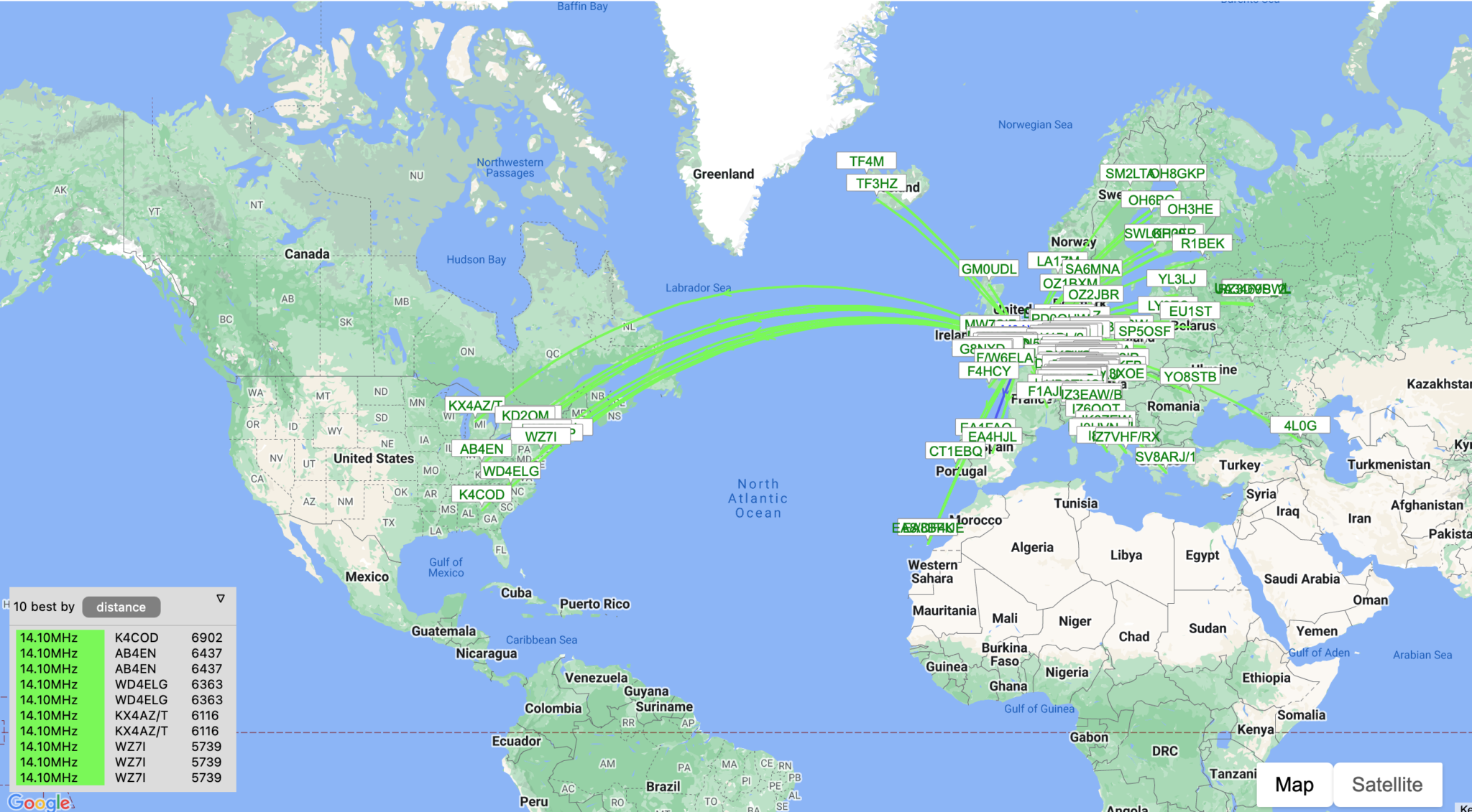
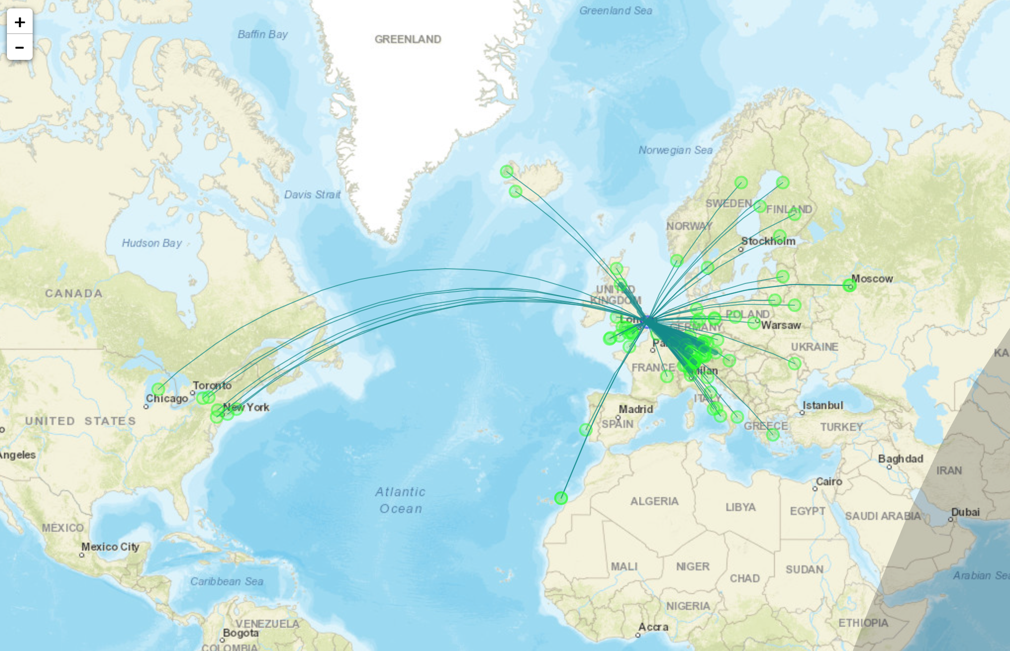
Map showing stations that heard M0AWS on WSPR

I used http://wspr.aprsinfo.com WSPR monitoring website to watch progress as the day went on and after 24hrs had been heard by a number of stations over 3000 miles away.

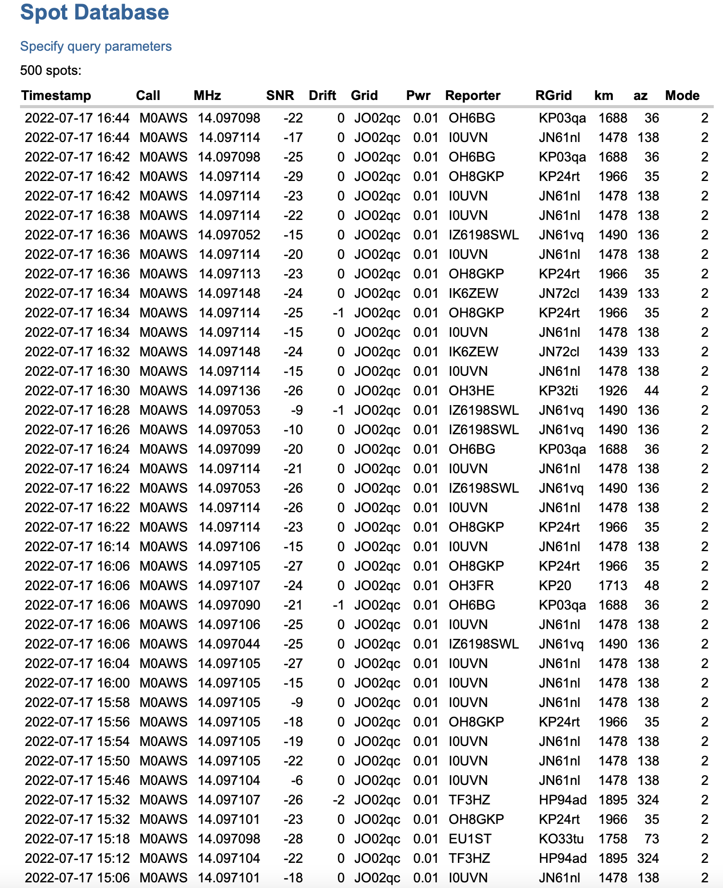
You can also get a more detailed view of reports from the WSPRnet website where you can query the database and create a detailed list of all decodes over a set period of time.

Detailed list of WSPR decodes

Since my EFHW Vertical is resonant on both 20m and 10m I’ll now run it for the next 24hrs on both bands to see what results I get.

More soon …

How low can you go?

Now that I’ve got my new radio shack up and running I decided to give my Icom IC-705 QRP rig an outing and see if I could work a distance of 2000 miles with 1w output.

This is something I’ve been wanting to do for a while but, only being able to sit at the picnic table in the garden or in the summer wasn’t particularly conducive to a long stint on the radio.

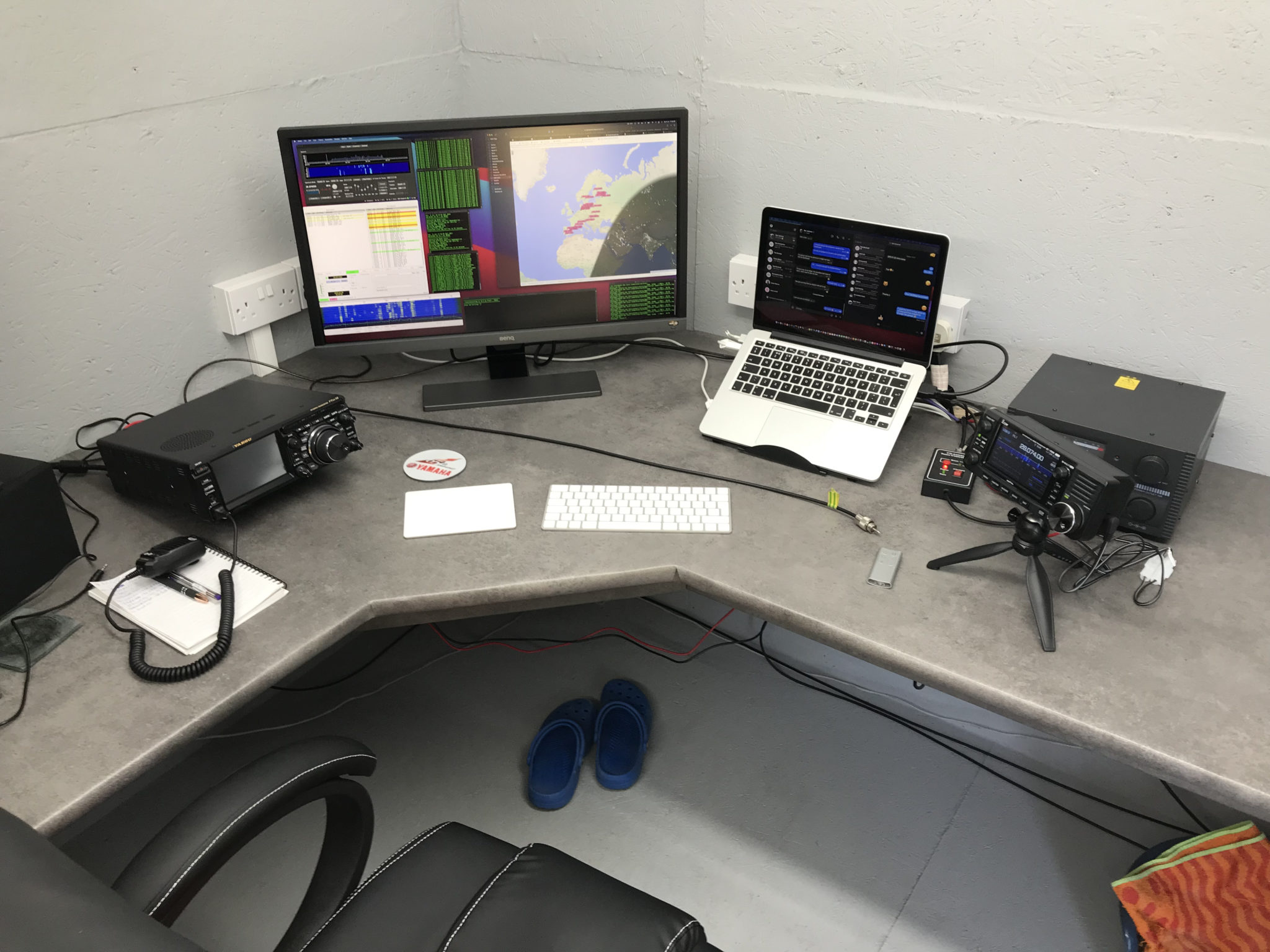
Icom IC-705 wirelessly connected to my MacBook Pro

For this challenge I decided to use FT4 or FT8, whichever was active on the bands. This is a great mode for QRP operations and can get a tiny signal through when other more traditional modes fail.

I used both my EFHW vertical for 20m/10m and my EFHW vertical for 30m that can also be tuned on most of the other HF bands too. This gave me most of the HF bands for the challenge.

Initially I worked a lot of stations in the 600-700 mile range, conditions weren’t brilliant and there was a lot of deep QSB.

My first notable distance QSO was with YO4DG near Mangalia Romania at 1383 miles, this equates to 0.72mW/Mile, my lowest mW/Mile achievement up until this point.

Not long afterwards I saw SV8DCY on the WSJTX waterfall, I wasn’t sure if he’d hear me or not but, I gave a call. To my surprise he came back and became the longest distance QSO for a short time. At 1485 Miles to Kalloni Lesvos Island, Greece this equates to a new low of 0.67mW/Mile.

I then went on to work a bunch of stations in the 1000 miles or less range for a while as conditions on the bands were up and down. It’s amazing how many times I got an answer from a station only for them to disappear completely before the QSO was completed.

The next contact of note was with CU3HN in the Azores, 1713 Miles at 0.58mW/Mile, a new lowest mW/Mile record set. it’s amazing how far you can get a signal with such a tiny amount of power.

RV6F in the Stavropol region of Russia was the next big mile marker, 1932 miles at 0.51mW/Mile. It took a number of attempts to get the QSO to complete as we kept losing each other due to the deep QSB that was between us on the 20m band but, with a little patience and persaverance we eventually got the QSO to complete and it was in the log.

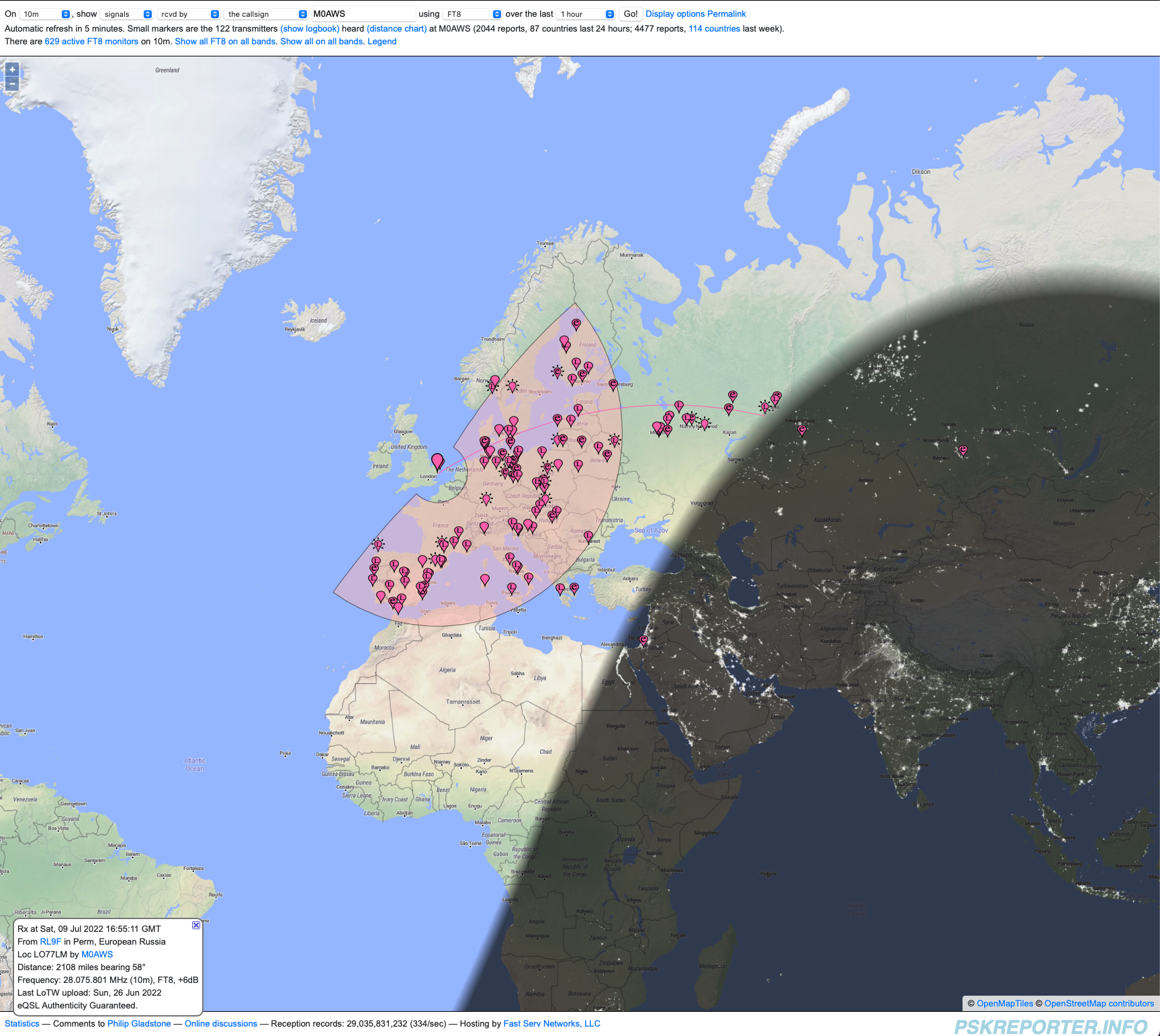
At this point I decided to switch over to the 10m band to see if it had opened up to more than just Europe. When I checked earlier there were only European stations being heard, most being well under 1000 miles. Sure enough the band had indeed opened up and I was hearing stations out to the east that were in excess of 2000 miles.

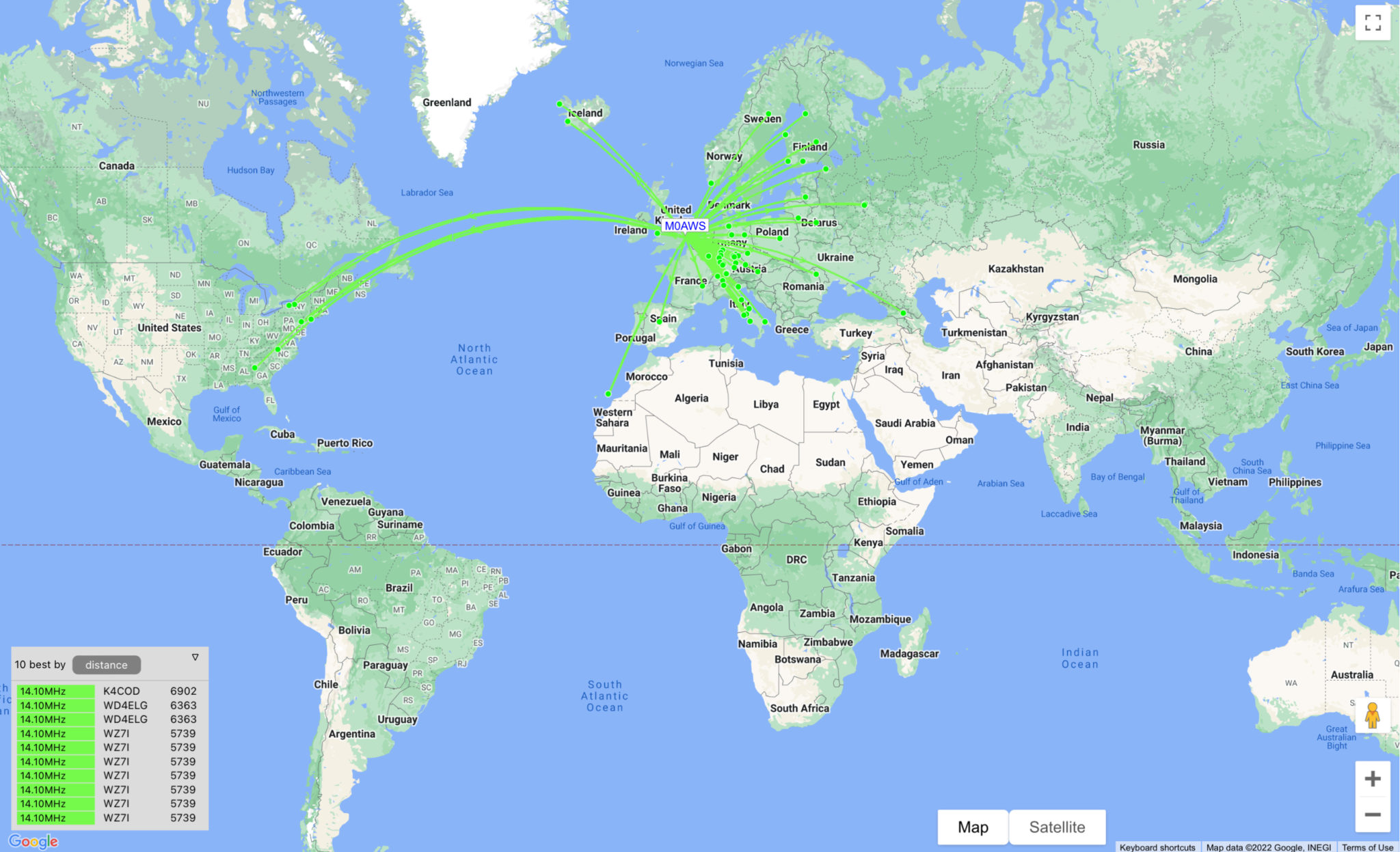
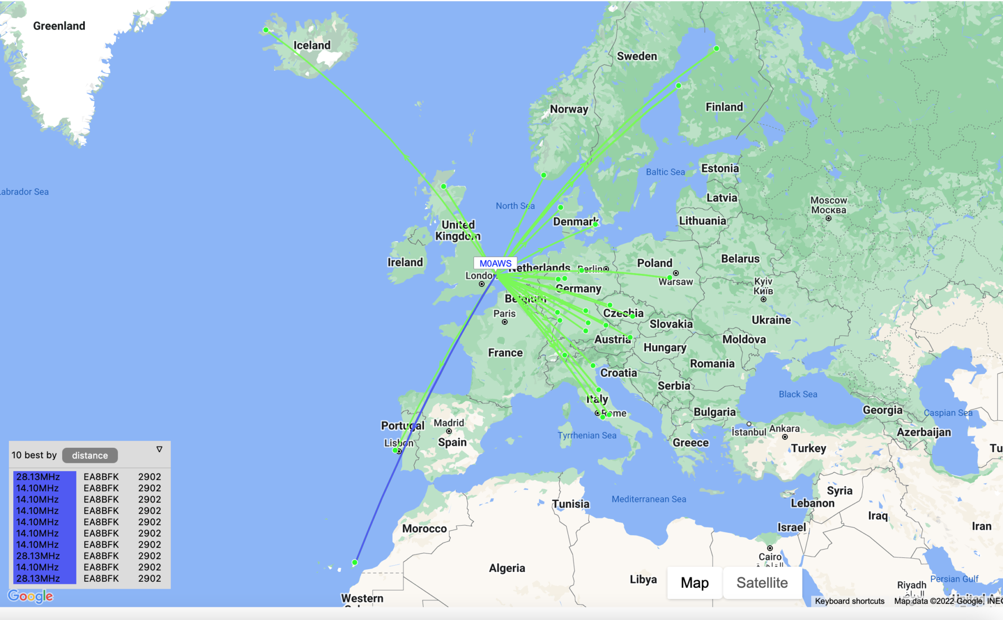
PSKReporter map showing signals heard on the 10m band

After tuning up and listening for a bit my first call was to RL9F in Perm Russia. This was the one that I’d been looking for, 2084 miles at 0.47mW/Mile this was the one that could complete the challenge.

After a few failed attempts due to deep QSB we eventually got a complete QSO in the log finishing the challenge.

2000 miles using 1w is a lot of fun, frustrating at times when you’re being heard by stations on the east coast USA but, none are answering your reply to their CQ calls.

PSKReporter has proven invaluable, being able to see who can hear you makes a big difference when trying to eek out the last mile when using next to no power.

In total 31 stations were worked over a 9 hour period, not huge numbers but, for many an M0AWS call sign isn’t exotic enough to answer and so many of my calls to stations were ignored. Sad really.

You can view all the log entries for the 2000 Mile 1 Watt challenge on my WSJTX Log.

So, what next? Well I guess it has to be 3000 miles or more using just 1w from my trusty Icom IC-705.

More soon …
300hz Filter for the Yaesu FTDX10

Since purchasing my new Begali Pearl morse key I’ve been wanting to install the 300hz CW filter into my Yaesu FTDX10. The radio comes standard from the factory with the 500z CW filter preinstalled however, being able to narrow the bandwidth down even further will help to reduce the ringing effect on noisy bands that often plaques CW Ops when trying to catch those very weak DX signals.

Since I had built up some free credit at ML&S by buying all my new radio equipment I decided to put it to good use and put it towards the cost of the optional 300hz filter for the radio.

In years past when I had a Yaesu FT1000MP I installed a full set of filters in it and it made quite a difference DXing on the 160/80/40m bands. Back then things like digital noise reduction (DNR) were in their infancy and so narrow filters were even more important than they are today.

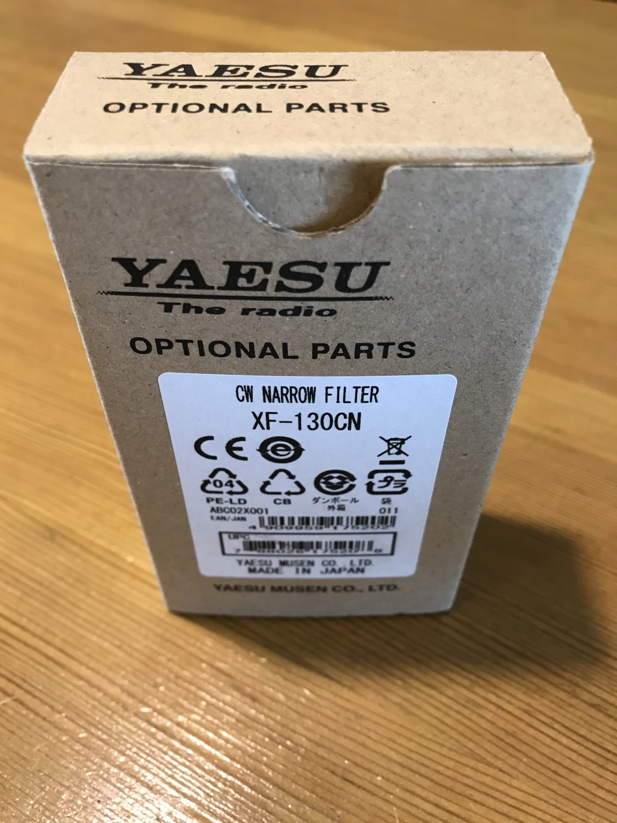
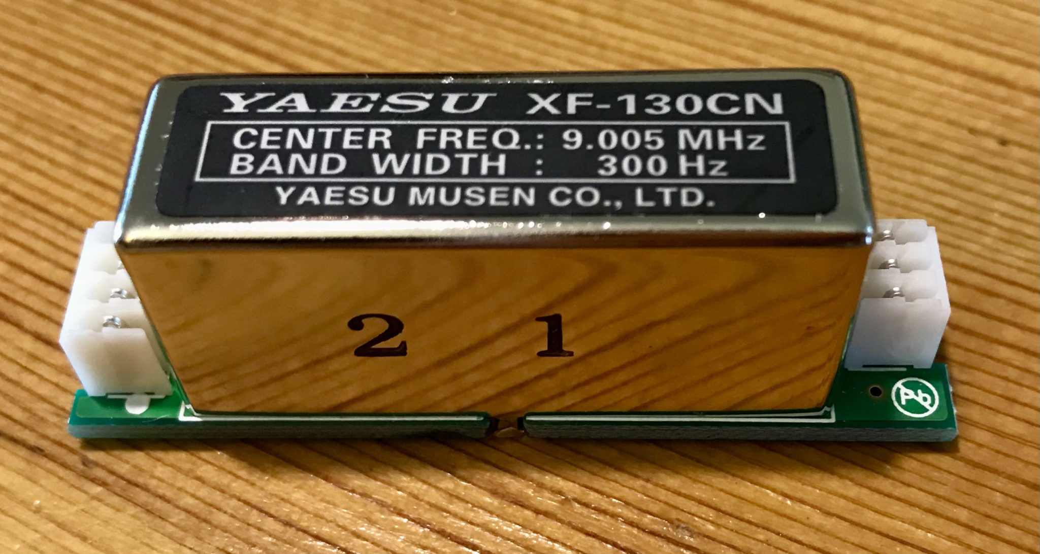
Yaesu XF-130CN 300hz CW Filter for the FTDX10

The FTDX10 300hz filter looked very similar to the ones I fitted in the FT1000MP and it doesn’t look like they’ve changed at all over the years.

Yaesu XF-130CN 300hz CW Filter

Removing the cover from the FTDX10 it’s immediately apparent where the filter goes. A neat little cutout in the RF shield draws your eye immediately to the spot.

Cutout in the RF shield for the optional 300hz filter

Fitting the filter is easy enough however, you do have to take care to move the little black wire to one side otherwise it gets caught under the filter and stops it from seating properly onto its connections. There’s not a lot of slack on the wire either so care is needed to not pull it too taught.

Note the black wire on the right hand site of the connections for the 300hz filter

I was surprised to see how small the standard 500hz filter is in comparison to the optional 300hz filter.

Optional 300hz filter next to the factory fitted 500hz filter

With the filter safely in position and seated perfectly I had the cover and 9 screws back on in no time at all and then got the radio powered up to check if the menu system had the option of a 300hz filter in CW mode.

FTDX10 CW filter menu with 300hz option

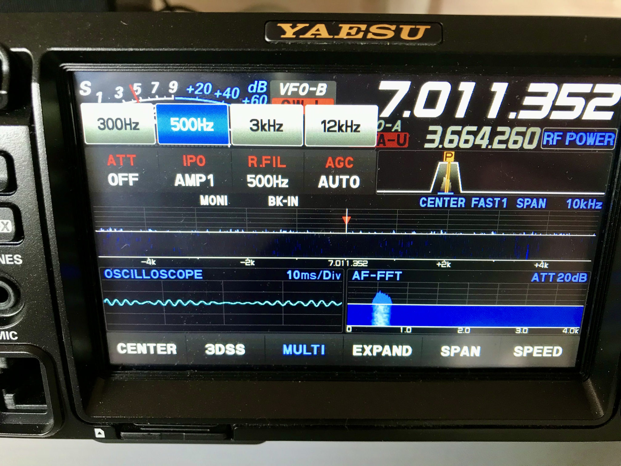
Getting on air the filter makes quite a difference to the amount of background noise when listening to weak DX stations. Adding DNR and APF to the equation removes all background noise completely with the 300hz filter making it possible to hear the weakest of CW stations and complete silence in-between.

The bands aren’t in particularly good shape today however, I tuned around on the 20m band and found W7SW in Phoenix Arizona calling CQ. He wasn’t particularly strong but, it was a good opportunity to experience the difference between the filters without any DNR or APF enhancement.

Short video showing difference between 500hz and 300hz filters with W7SW calling CQ

Unfortunately W7SW disappeared before I could make another short video with the DNR and APF on to show the difference. I’ll revisit this again soon and get some video snippets up showing the difference the optional 300hz filter makes with DNR and APF.

More soon …

An evening of FT8 on the 40m Band

I spent the evening/early morning trying some FT8 on the 40m band taking advantage of the grey line and night time propagation. It’s been a while since I’ve stayed up late to catch some DX on 40m and it brought back memories of the all nighters I used to do when I was on air as F5VKM in France.

The 40m band has always been one of my favourites, there’s always great DX to be had when the band is open and on the grey line the world really is your oyster.

I’ve always been a huge fan of CW on 40m, there are some great seasoned op’s on the band and it’s always a real pleasure to QSO with them on the key. This time I decided to see what could be achieved with FT8 and 22w of power from my Yaesu FTDX10, a combination that should give me global reach.

Setting up at just past 6pm on May 9th 2022 the band was already busy with European stations, lots of them! There was no room to squeeze in and call CQ, the FT8 section of the band was packed with signals filling the allocation completely with many calling over the top of each other.

I decided to take my normal stance of search and pounce to get the stations I want to work rather than just working the masses endlessly.

I initially worked a bunch of Russian stations ranging from 1200 to 2200 miles out, good distances were easily achievable even though we were still in full daylight.

My home-brew multi-band vertical antenna worked well on 40m

In amongst the throng of FT8 stations I spotted UN3P, Vladimir in Karaganda Kazakhstan, not a country I have worked a lot since getting back on air and at 3013 miles it’s a good distance to achieve on 40m whilst still in broad daylight.

I gave a call to his CQ and he came straight back with an SNR report of -20dB, I sent him a report of -12dB so there was some 8dB difference between us. Considering I was only using 22w of power in broad daylight I was happy with the report. Of course I’ve no idea how much power he was using but, my signal was 6.63mW/Mile, not the lowest I ever had but, not the biggest either.

I worked a bunch more RA9/UB9 stations in the 2000-3000 mile range and then started hearing the Australian stations on the early grey line. Initially their signals were suffering some deep QSB but, it wasn’t long until their signals were constant and stable.

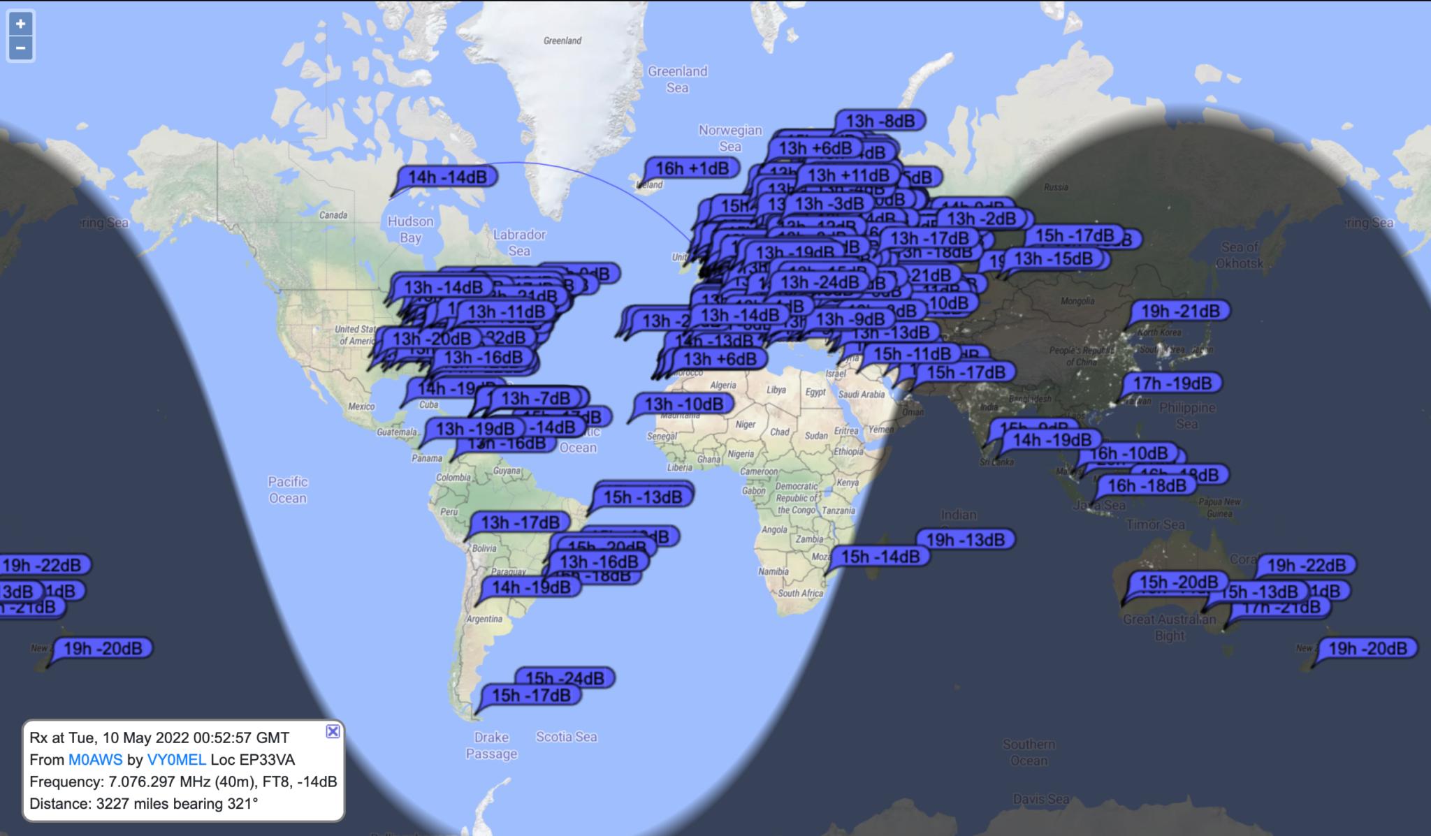
All the stations that heard M0AWS 09/05/22 – 10/05/22 on 40m

Ian, VK3VDX in Victoria was the first station from Oz in the log at -19dB/-20dB, pretty even SNR reports. At 10451 miles it equates to 2.10mW/Mile.

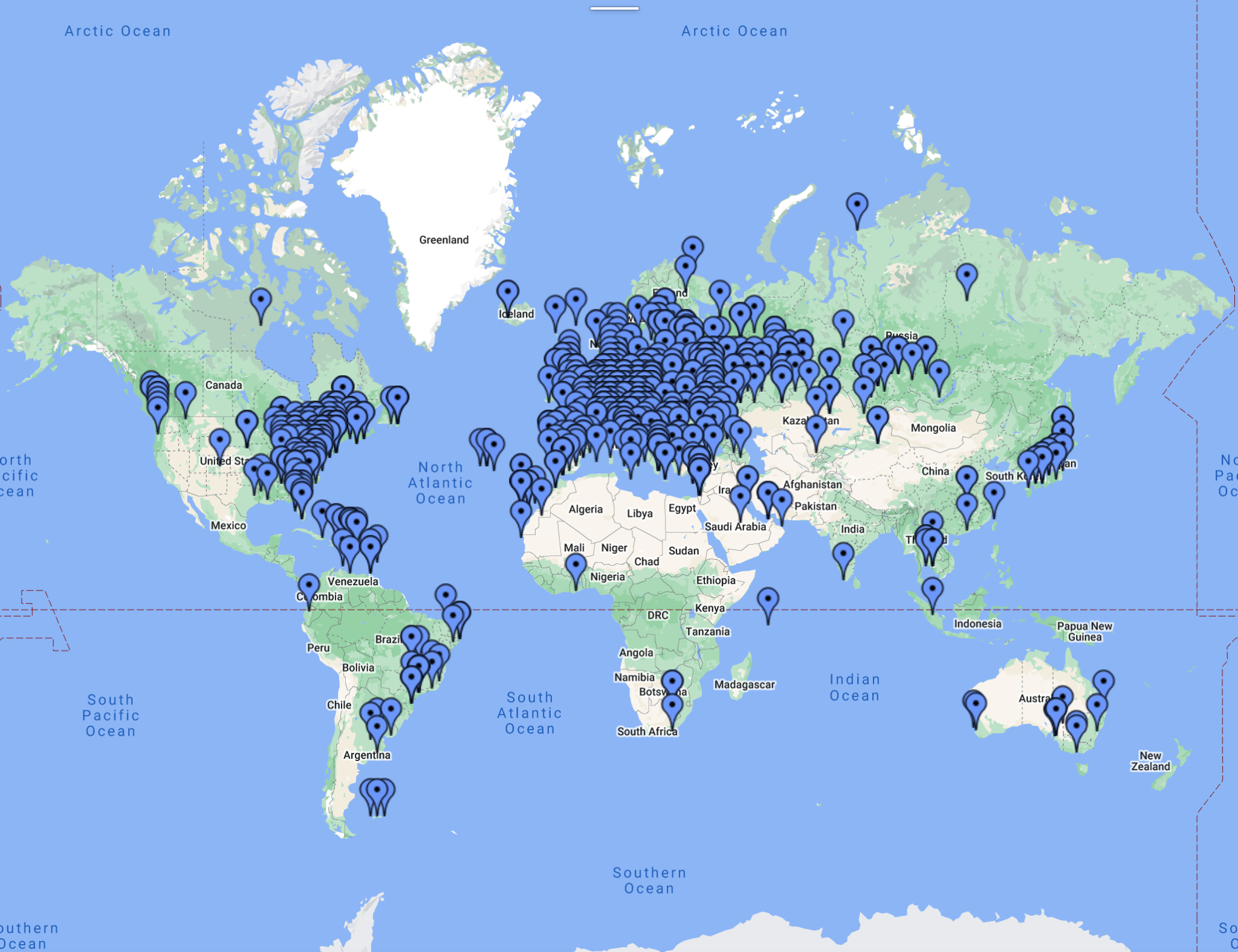
Closely following was John, VK5PO in Mallala South Australia, much stronger signals this time at -10dB/-14dB, 2.19mW/mile over a total distance of 10028 miles.

VK5PO Mallala South Australia

As darkness replaced light the propagation swung west with east coast USA and Canadian stations dropping in to the East coast of the U.K.

John, VO1BE was the first north American station in the log with -1dB/+1dB SNR reports. To be +1dB in Canada with just 22w really is quite impressive. I’m guessing he has a very low background noise level.

I worked a bunch of East Coast USA stations and then PY2GZ popped up on the waterfall. From my QTH I have a clear view South East to South West across flat ground for miles and so it’s normally pretty easy to work stations in that zone and this evening was no different. First call was answered and -10dB/-17dB SNR reports were exchanged, 3.68mW/mile over 5965 miles.

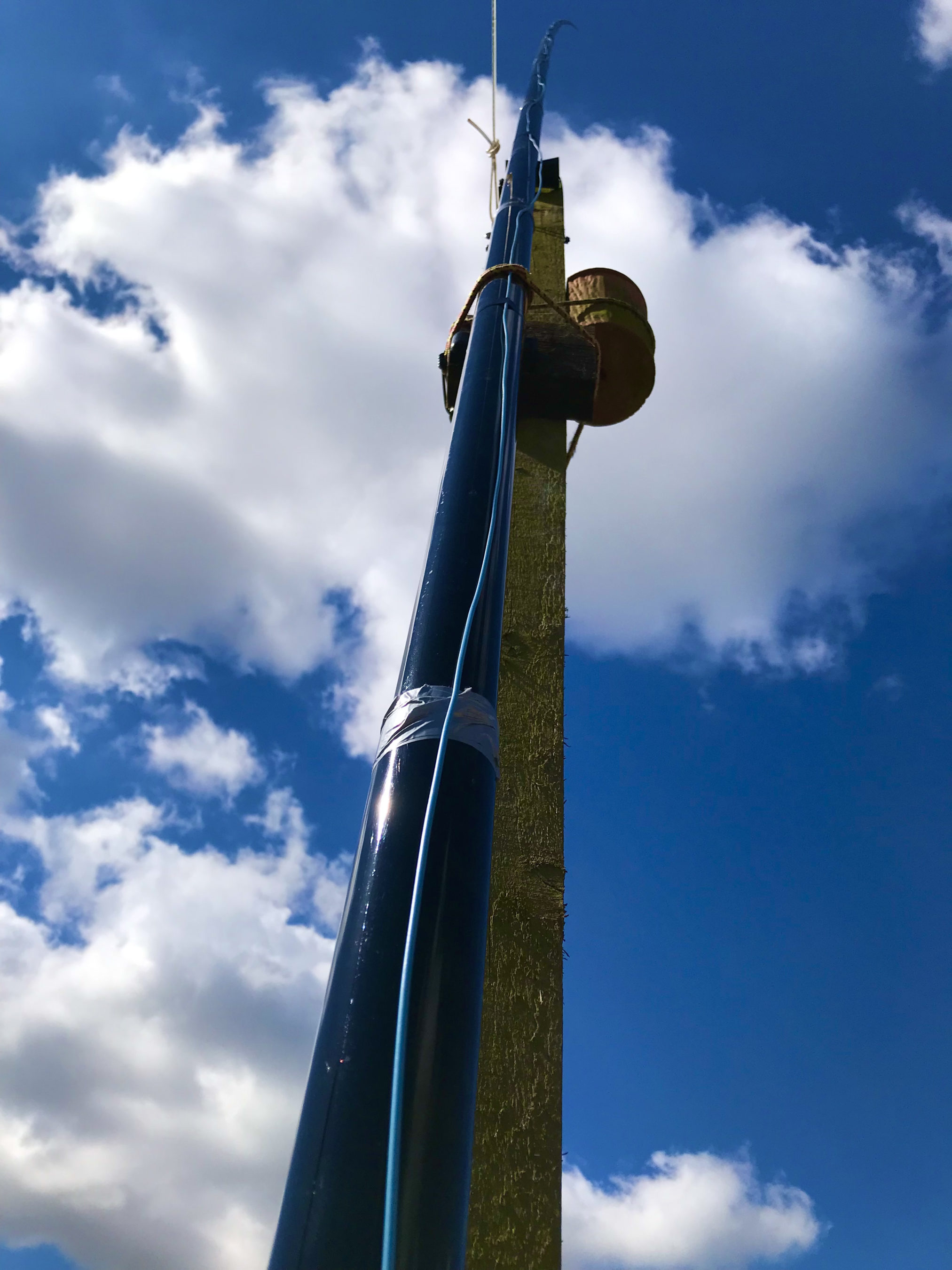
My 14.81m tall home brew vertical works superbly on the 40m band with tuning handled by my CG3000 Remote Auto Tuner. This is actually my 30m band EFHW vertical antenna but, removing the 49:1 Unun and replacing it with the CG3000 has made this antenna much more versatile.

CG3000 Remote Auto Tuner connected to the 14.81m vertical antenna and ground system

The next station in the log was BG0BBB in Xinjiang China with -9dB/-18dB SNR reports exchanged. China is always a hard location for me to get into for some reason so, I was glad to get another Chinese HAM into the log.

BG0BBB Xinjiang China

As the propagation started to swing westerly I got 8P4JP in Bridgetown Barbados into the log. It took a few calls to get the exchange completed due to very deep QSB between us but, with some perseverance the contact was completed successfully and I had a new one in the log!

I continued to work a flurry of East Coast USA, Brazilian and Puerto Ricon stations one after the other until suddenly stations from the east started coming in again.

First from the east was Igor, 4L1FL from Tbilisi Georgia, another new one for me that somehow seems to escape me every time I come across Georgian stations on the bands.

4L1FL Tbilisi Georgia

UN7JO in Ust-Kamenogorsk Kazakhstan was loud with me at -5dB SNR although I only got -21dB SNR back, some 16dB difference across the path of 3386 Miles.

One station of particular interest was VY0MEL, Julien in Rankin Inlet, Nunavut Northern Canada. This is the most northern Canadian station I’ve worked in a long time and it was great to get him in the log. His QRZ page is worth a read, he works at a mine in Nunavut on a 14 day rotation and so has a fair bit of time for HAM radio. Using just a dipole that is strung between two shipping containers and only 60cm above the snow in the centre he was a good signal at -19dB here in the U.K, especially considering he was still in broad daylight.

VY0MEL Rankin Inlet, Nunavut Northern Canada

Needless to say I had a fun filled evening/early morning on the 40m band, once again it didn’t disappoint and I got a couple of new countries in the log. I think the next late night will have to be a CW evening on 40m to see how well I do in comparison.

The full list of stations worked over 9th-10th May 2022 using FT8 on the 40m band can be viewed in my WSJT-X log in glorious technicolour with distances and mW/mile figures for every contact.

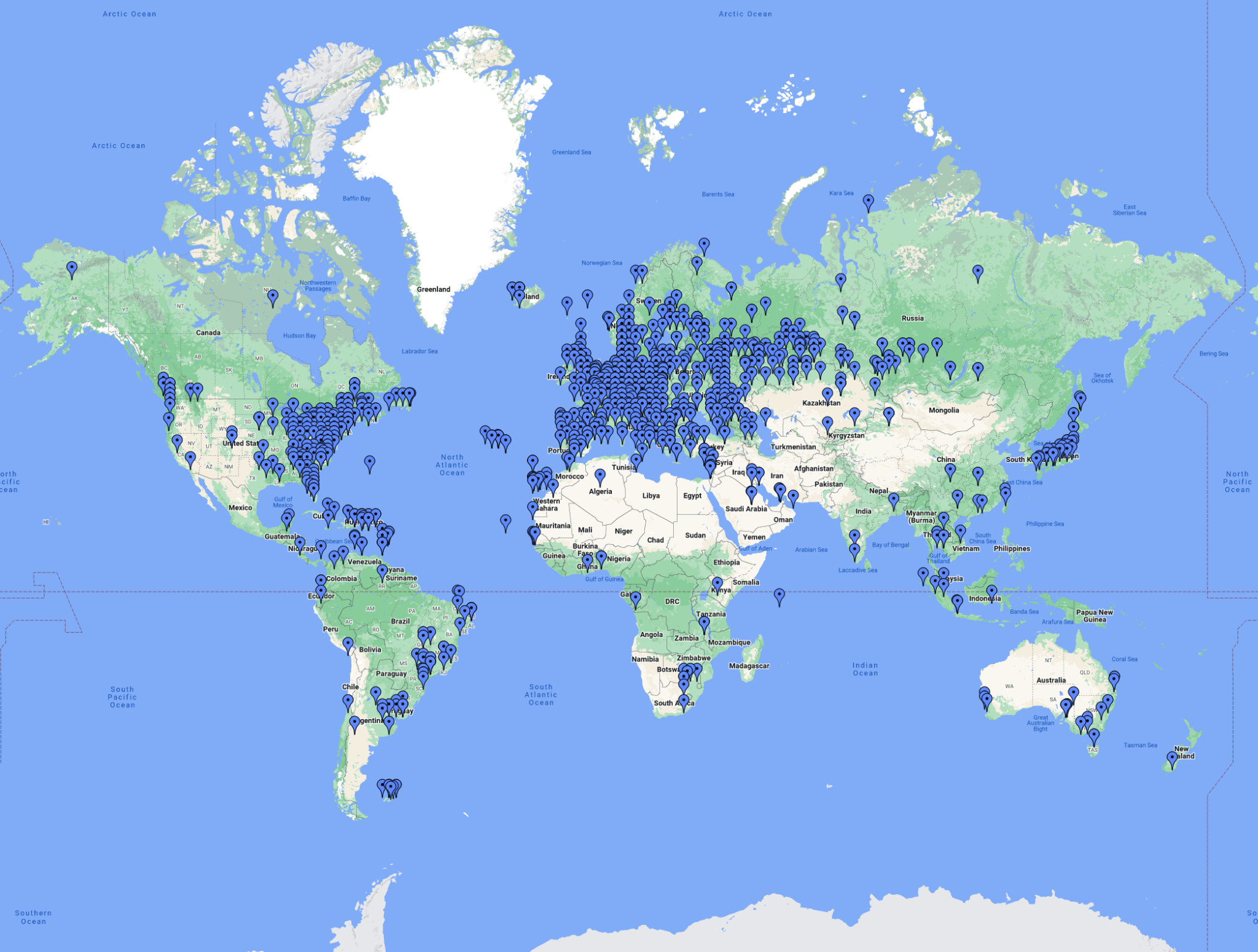
Map showing all FT4/FT8 stations worked up to 10/05/22 all bands

More soon …
80m Band NVIS Antenna Experiment

Following on from my 40m band NVIS antenna experiment I ran the same series of tests on the 80m band to see how well the NVIS antenna works.

Being only 30m long the antenna isn’t very well suited to the low bands but, with the tiny garden we have here in the U.K. and the anti-antenna neighbours it’s the best I can do.

I started off looking for SSB contacts only to find no one on the band. I eventually found G8MNY calling CQ from Croydon south of London. He was a huge 5/9+20db with me so I was hopeful that he’d hear me.

Tuning up the antenna on 3.710Mhz and setting the O/P to 40w I gave him a call and got an immediate response. We ended up chatting for around 30mins with ease, the band wasn’t too noisy and Jon was running 400w so he was a solid signal with me. My 40w got me a 5/8 report which I was very happy with.

Once we cleared I tuned around the band and even called CQ a few times, but there was nothing to be heard.

I went and had something to eat and then returned to the shack before the greyline, the band was a little more lively and so I switched over to FT8 mode and started working stations.

Stations initially heard on FT8 whilst still in daylight

I was really quite surprised how many stations I could hear and make contact with even though I was still in daylight. The effect of the greyline really is quite pronounced.

Stations that heard me on FT8 whilst still in daylight

I was being heard by a good number of continental stations even though I was still in daylight. Signal strengths were good and I was soon working stations one after another with ease.

As the night drew closer and the U.K. moved into darkness stations further east started appearing on the WSJT-X window and I was surprised how many I was able to work considering how low and short the antenna is for this band.

German stations were always the strongest throughout the test which is to be expected with an NVIS antenna as they are just across the north sea as the crow flies.

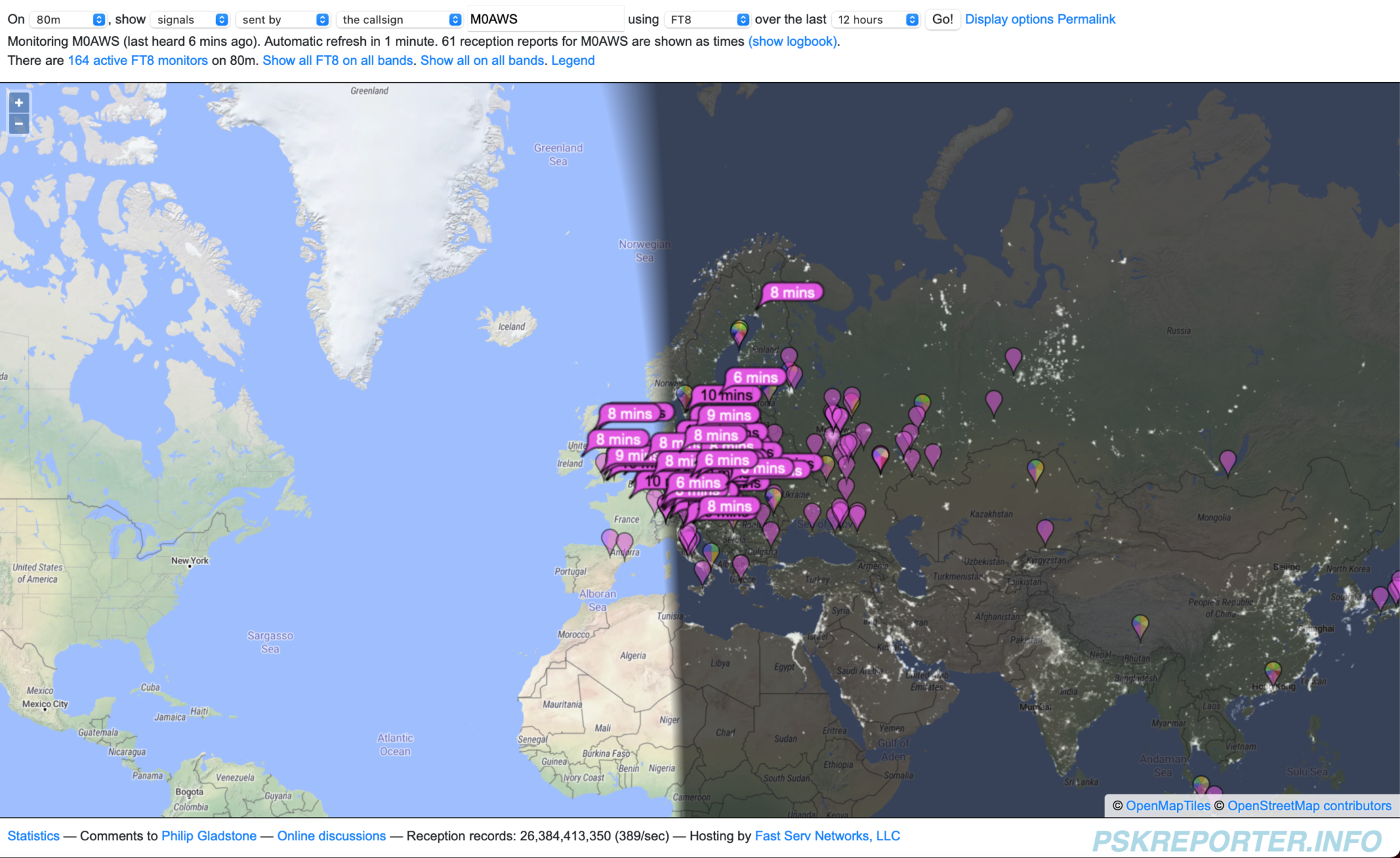
Map showing all stations heard on FT8 during 80m NVIS antenna experiment

By the end of the evening I’d heard a good number of stations with the most distant being north of the Kazakhstan/Mongolian border as shown on the map above.

All stations that heard M0AWS on FT8 throughout the NVIS antenna experiment

I was pleasantly surprised at how many stations were hearing me throughout the test, getting as far south as the islands off the coast of north Africa and well into Russia was amazing for a horizontal antenna that is only 4m-5m above the ground.

Map of all stations worked during the 80m NVIS antenna experiment

The number of contacts was nowhere near as prolific as during the 40m experiment mainly due to the fact that the band wasn’t as busy however, the contact pattern was very similar to that on 40m with the most distant station being R2EA/P just south east of Moscow at 1544 miles.

European coverage was very good but, sadly I didn’t hear many U.K. stations and so I’m not sure how well my Inter-G coverage will be. Perhaps another test during the day when conditions are better will shed some more light on this.

Overall I’m very happy with the antenna performance on the 80m band, it’ll certainly be ideal for European chat during the summer months and hopefully inter-G will be good too.

Next will be a test on 160m, this could be interesting!

More soon …

adi2html v0.6 release

Following on from the adi2html v0.5 release I’ve now added a little more code to include a map of the contacts detailed in the wsjtx_log.adi file so that there is a visual representation of the data included in the webpage. (Map must be generated externally and JPEG/GIF/PNG uploaded to website to be included in the webpage).

See my WSJT-X log here

Just to recap, adi2html generates a HTML webpage from the wsjtx_log.adi file so that the log can be presented in a palatable format on a website.

As before the code can be downloaded using the link below.

If you use my code please consider leaving the footer in place so I get some credit, thanks!